Guorui Zhong - Customization of Seurat plots using ggplot2

Packages

library(here)
library(tidyverse)
library(Seurat)
library(SingleR)
library(ggrepel)
library(ggthemes)
library(ggnewscale)
library(tidyverse)
library(scCustomize)
library(viridis)
library(RColorBrewer)
library(gridExtra)
library(ComplexHeatmap)
library(dittoSeq)
library(Scillus)

UMAP

Load Seurat object

### Load data
load(here("learn", "2023_scRNA_Seurat", "pbmc_tutorial_singleR.RData"))
load(here("learn", "2023_scRNA_Seurat", "sce.anno.RData"))
load(here("learn", "2023_scRNA_Seurat", "all_markers.RData"))
top5 <- all_markers |> group_by(cluster) |> top_n(5, avg_log2FC)

### Check data
head(pbmc, 2)
##                  orig.ident nCount_RNA nFeature_RNA percent.mt percent.HB
## AAACATACAACCAC-1     pbmc3k       2419          779   3.017776          0
## AAACATTGAGCTAC-1     pbmc3k       4903         1352   3.793596          0
##                  RNA_snn_res.0.5 seurat_clusters  labels
## AAACATACAACCAC-1               0               0 T_cells
## AAACATTGAGCTAC-1               3               3  B_cell
head(sce2, 2)
##                         orig.ident nCount_RNA nFeature_RNA percent.mt
## K16733_AAACATACTCGTTT-1     K16733       2464          965  12.662338
## K16733_AAAGCAGAACGTTG-1     K16733       7145         1919   2.449265
##                         percent.rp percent.HB RNA_snn_res.0.5 seurat_clusters
## K16733_AAACATACTCGTTT-1   13.35227          0              11              11
## K16733_AAAGCAGAACGTTG-1   36.72498          0               3               3
##                         sampel sample group    globalC       anno
## K16733_AAACATACTCGTTT-1    P01    P01    PT        Epi        Epi
## K16733_AAAGCAGAACGTTG-1    P01    P01    PT Fibroblast Fibroblast
head(top5)
## # A tibble: 6 × 7
## # Groups:   cluster [2]
##       p_val avg_log2FC pct.1 pct.2 p_val_adj cluster gene      
##       <dbl>      <dbl> <dbl> <dbl>     <dbl> <fct>   <chr>     
## 1 2.43e- 67       3.05 0.172 0.079 1.26e- 62 0       REG4      
## 2 3.38e- 51       3.19 0.069 0.019 1.76e- 46 0       BPIFB1    
## 3 5.32e- 30       3.71 0.031 0.007 2.76e- 25 0       FABP1     
## 4 6.37e- 21       2.79 0.018 0.003 3.31e- 16 0       SLC9A4    
## 5 1.65e- 20       2.70 0.017 0.003 8.56e- 16 0       AC073218.2
## 6 2.51e-112       3.57 0.132 0.023 1.30e-107 1       SPRR1A

Default seurat UMAP

# View the UMAP
DimPlot(pbmc, group.by = c("seurat_clusters", "labels"), reduction = "umap")

UMAP with ggplot2

# Find the UMAP data
str(pbmc)
## Formal class 'Seurat' [package "SeuratObject"] with 13 slots
##   ..@ assays      :List of 1
##   .. ..$ RNA:Formal class 'Assay' [package "SeuratObject"] with 8 slots
##   .. .. .. ..@ counts       :Formal class 'dgCMatrix' [package "Matrix"] with 6 slots
##   .. .. .. .. .. ..@ i       : int [1:2238732] 29 73 80 148 163 184 186 227 229 230 ...
##   .. .. .. .. .. ..@ p       : int [1:2639] 0 779 2131 3260 4220 4741 5522 6304 7094 7626 ...
##   .. .. .. .. .. ..@ Dim     : int [1:2] 13714 2638
##   .. .. .. .. .. ..@ Dimnames:List of 2
##   .. .. .. .. .. .. ..$ : chr [1:13714] "AL627309.1" "AP006222.2" "RP11-206L10.2" "RP11-206L10.9" ...
##   .. .. .. .. .. .. ..$ : chr [1:2638] "AAACATACAACCAC-1" "AAACATTGAGCTAC-1" "AAACATTGATCAGC-1" "AAACCGTGCTTCCG-1" ...
##   .. .. .. .. .. ..@ x       : num [1:2238732] 1 1 2 1 1 1 1 41 1 1 ...
##   .. .. .. .. .. ..@ factors : list()
##   .. .. .. ..@ data         :Formal class 'dgCMatrix' [package "Matrix"] with 6 slots
##   .. .. .. .. .. ..@ i       : int [1:2238732] 29 73 80 148 163 184 186 227 229 230 ...
##   .. .. .. .. .. ..@ p       : int [1:2639] 0 779 2131 3260 4220 4741 5522 6304 7094 7626 ...
##   .. .. .. .. .. ..@ Dim     : int [1:2] 13714 2638
##   .. .. .. .. .. ..@ Dimnames:List of 2
##   .. .. .. .. .. .. ..$ : chr [1:13714] "AL627309.1" "AP006222.2" "RP11-206L10.2" "RP11-206L10.9" ...
##   .. .. .. .. .. .. ..$ : chr [1:2638] "AAACATACAACCAC-1" "AAACATTGAGCTAC-1" "AAACATTGATCAGC-1" "AAACCGTGCTTCCG-1" ...
##   .. .. .. .. .. ..@ x       : num [1:2238732] 1.64 1.64 2.23 1.64 1.64 ...
##   .. .. .. .. .. ..@ factors : list()
##   .. .. .. ..@ scale.data   : num [1:2000, 1:2638] -0.8556 -0.2773 1.4947 -0.0463 -0.4658 ...
##   .. .. .. .. ..- attr(*, "dimnames")=List of 2
##   .. .. .. .. .. ..$ : chr [1:2000] "ISG15" "CPSF3L" "MRPL20" "ATAD3C" ...
##   .. .. .. .. .. ..$ : chr [1:2638] "AAACATACAACCAC-1" "AAACATTGAGCTAC-1" "AAACATTGATCAGC-1" "AAACCGTGCTTCCG-1" ...
##   .. .. .. ..@ assay.orig   : NULL
##   .. .. .. ..@ var.features : chr [1:2000] "PPBP" "LYZ" "S100A9" "IGLL5" ...
##   .. .. .. ..@ meta.features:'data.frame':   13714 obs. of  5 variables:
##   .. .. .. .. ..$ vst.mean                 : num [1:13714] 0.00341 0.00114 0.0019 0.00114 0.00682 ...
##   .. .. .. .. ..$ vst.variance             : num [1:13714] 0.0034 0.00114 0.00189 0.00114 0.00678 ...
##   .. .. .. .. ..$ vst.variance.expected    : num [1:13714] 0.00365 0.00114 0.00197 0.00114 0.00748 ...
##   .. .. .. .. ..$ vst.variance.standardized: num [1:13714] 0.933 0.992 0.963 0.992 0.906 ...
##   .. .. .. .. ..$ vst.variable             : logi [1:13714] FALSE FALSE FALSE FALSE FALSE FALSE ...
##   .. .. .. ..@ misc         : list()
##   .. .. .. ..@ key          : chr "rna_"
##   ..@ meta.data   :'data.frame': 2638 obs. of  8 variables:
##   .. ..$ orig.ident     : Factor w/ 1 level "pbmc3k": 1 1 1 1 1 1 1 1 1 1 ...
##   .. ..$ nCount_RNA     : num [1:2638] 2419 4903 3147 2639 980 ...
##   .. ..$ nFeature_RNA   : int [1:2638] 779 1352 1129 960 521 781 782 790 532 550 ...
##   .. ..$ percent.mt     : num [1:2638] 3.02 3.79 0.89 1.74 1.22 ...
##   .. ..$ percent.HB     : num [1:2638] 0 0 0 0 0 0 0 0 0 0 ...
##   .. ..$ RNA_snn_res.0.5: Factor w/ 9 levels "0","1","2","3",..: 1 4 3 2 7 3 5 5 5 6 ...
##   .. ..$ seurat_clusters: Factor w/ 9 levels "0","1","2","3",..: 1 4 3 2 7 3 5 5 5 6 ...
##   .. ..$ labels         : chr [1:2638] "T_cells" "B_cell" "T_cells" "Monocyte" ...
##   ..@ active.assay: chr "RNA"
##   ..@ active.ident: Factor w/ 9 levels "0","1","2","3",..: 1 4 3 2 7 3 5 5 5 6 ...
##   .. ..- attr(*, "names")= chr [1:2638] "AAACATACAACCAC-1" "AAACATTGAGCTAC-1" "AAACATTGATCAGC-1" "AAACCGTGCTTCCG-1" ...
##   ..@ graphs      :List of 2
##   .. ..$ RNA_nn :Formal class 'Graph' [package "SeuratObject"] with 7 slots
##   .. .. .. ..@ assay.used: chr "RNA"
##   .. .. .. ..@ i         : int [1:52760] 0 6 102 203 213 229 292 451 547 618 ...
##   .. .. .. ..@ p         : int [1:2639] 0 33 50 64 80 87 103 139 155 162 ...
##   .. .. .. ..@ Dim       : int [1:2] 2638 2638
##   .. .. .. ..@ Dimnames  :List of 2
##   .. .. .. .. ..$ : chr [1:2638] "AAACATACAACCAC-1" "AAACATTGAGCTAC-1" "AAACATTGATCAGC-1" "AAACCGTGCTTCCG-1" ...
##   .. .. .. .. ..$ : chr [1:2638] "AAACATACAACCAC-1" "AAACATTGAGCTAC-1" "AAACATTGATCAGC-1" "AAACCGTGCTTCCG-1" ...
##   .. .. .. ..@ x         : num [1:52760] 1 1 1 1 1 1 1 1 1 1 ...
##   .. .. .. ..@ factors   : list()
##   .. ..$ RNA_snn:Formal class 'Graph' [package "SeuratObject"] with 7 slots
##   .. .. .. ..@ assay.used: chr "RNA"
##   .. .. .. ..@ i         : int [1:194424] 0 6 102 136 187 203 229 292 421 446 ...
##   .. .. .. ..@ p         : int [1:2639] 0 62 120 170 240 287 379 453 533 573 ...
##   .. .. .. ..@ Dim       : int [1:2] 2638 2638
##   .. .. .. ..@ Dimnames  :List of 2
##   .. .. .. .. ..$ : chr [1:2638] "AAACATACAACCAC-1" "AAACATTGAGCTAC-1" "AAACATTGATCAGC-1" "AAACCGTGCTTCCG-1" ...
##   .. .. .. .. ..$ : chr [1:2638] "AAACATACAACCAC-1" "AAACATTGAGCTAC-1" "AAACATTGATCAGC-1" "AAACCGTGCTTCCG-1" ...
##   .. .. .. ..@ x         : num [1:194424] 1 0.1111 0.1765 0.0811 0.0811 ...
##   .. .. .. ..@ factors   : list()
##   ..@ neighbors   : list()
##   ..@ reductions  :List of 3
##   .. ..$ pca :Formal class 'DimReduc' [package "SeuratObject"] with 9 slots
##   .. .. .. ..@ cell.embeddings           : num [1:2638, 1:50] -5.84 -2.56 -1.64 13.29 -2.15 ...
##   .. .. .. .. ..- attr(*, "dimnames")=List of 2
##   .. .. .. .. .. ..$ : chr [1:2638] "AAACATACAACCAC-1" "AAACATTGAGCTAC-1" "AAACATTGATCAGC-1" "AAACCGTGCTTCCG-1" ...
##   .. .. .. .. .. ..$ : chr [1:50] "PC_1" "PC_2" "PC_3" "PC_4" ...
##   .. .. .. ..@ feature.loadings          : num [1:2000, 1:50] 0.01091 0.11663 0.11569 -0.00853 -0.01632 ...
##   .. .. .. .. ..- attr(*, "dimnames")=List of 2
##   .. .. .. .. .. ..$ : chr [1:2000] "PPBP" "LYZ" "S100A9" "IGLL5" ...
##   .. .. .. .. .. ..$ : chr [1:50] "PC_1" "PC_2" "PC_3" "PC_4" ...
##   .. .. .. ..@ feature.loadings.projected: num[0 , 0 ] 
##   .. .. .. ..@ assay.used                : chr "RNA"
##   .. .. .. ..@ global                    : logi FALSE
##   .. .. .. ..@ stdev                     : num [1:50] 7.05 4.5 3.87 3.75 3.15 ...
##   .. .. .. ..@ jackstraw                 :Formal class 'JackStrawData' [package "SeuratObject"] with 4 slots
##   .. .. .. .. .. ..@ empirical.p.values     : num [1:2000, 1:20] 0.0005 0 0 0.0035 0 0 0.01 0 0.0135 0 ...
##   .. .. .. .. .. .. ..- attr(*, "dimnames")=List of 2
##   .. .. .. .. .. .. .. ..$ : chr [1:2000] "PPBP" "LYZ" "S100A9" "IGLL5" ...
##   .. .. .. .. .. .. .. ..$ : chr [1:20] "PC1" "PC2" "PC3" "PC4" ...
##   .. .. .. .. .. ..@ fake.reduction.scores  : num [1:2000, 1:20] -0.003524 0.000285 -0.000627 0.002054 0.000959 ...
##   .. .. .. .. .. ..@ empirical.p.values.full: logi [1, 1] NA
##   .. .. .. .. .. ..@ overall.p.values       : num [1:20, 1:2] 1 2 3 4 5 6 7 8 9 10 ...
##   .. .. .. .. .. .. ..- attr(*, "dimnames")=List of 2
##   .. .. .. .. .. .. .. ..$ : NULL
##   .. .. .. .. .. .. .. ..$ : chr [1:2] "PC" "Score"
##   .. .. .. ..@ misc                      :List of 1
##   .. .. .. .. ..$ total.variance: num 1734
##   .. .. .. ..@ key                       : chr "PC_"
##   .. ..$ umap:Formal class 'DimReduc' [package "SeuratObject"] with 9 slots
##   .. .. .. ..@ cell.embeddings           : num [1:2638, 1:2] -4.58 -2.81 -1.68 12.69 -9.83 ...
##   .. .. .. .. ..- attr(*, "scaled:center")= num [1:2] -0.0395 -1.1523
##   .. .. .. .. ..- attr(*, "dimnames")=List of 2
##   .. .. .. .. .. ..$ : chr [1:2638] "AAACATACAACCAC-1" "AAACATTGAGCTAC-1" "AAACATTGATCAGC-1" "AAACCGTGCTTCCG-1" ...
##   .. .. .. .. .. ..$ : chr [1:2] "UMAP_1" "UMAP_2"
##   .. .. .. ..@ feature.loadings          : num[0 , 0 ] 
##   .. .. .. ..@ feature.loadings.projected: num[0 , 0 ] 
##   .. .. .. ..@ assay.used                : chr "RNA"
##   .. .. .. ..@ global                    : logi TRUE
##   .. .. .. ..@ stdev                     : num(0) 
##   .. .. .. ..@ jackstraw                 :Formal class 'JackStrawData' [package "SeuratObject"] with 4 slots
##   .. .. .. .. .. ..@ empirical.p.values     : num[0 , 0 ] 
##   .. .. .. .. .. ..@ fake.reduction.scores  : num[0 , 0 ] 
##   .. .. .. .. .. ..@ empirical.p.values.full: num[0 , 0 ] 
##   .. .. .. .. .. ..@ overall.p.values       : num[0 , 0 ] 
##   .. .. .. ..@ misc                      : list()
##   .. .. .. ..@ key                       : chr "UMAP_"
##   .. ..$ tsne:Formal class 'DimReduc' [package "SeuratObject"] with 9 slots
##   .. .. .. ..@ cell.embeddings           : num [1:2638, 1:2] -11.1 -36.27 1.96 37.46 -20.88 ...
##   .. .. .. .. ..- attr(*, "dimnames")=List of 2
##   .. .. .. .. .. ..$ : chr [1:2638] "AAACATACAACCAC-1" "AAACATTGAGCTAC-1" "AAACATTGATCAGC-1" "AAACCGTGCTTCCG-1" ...
##   .. .. .. .. .. ..$ : chr [1:2] "tSNE_1" "tSNE_2"
##   .. .. .. ..@ feature.loadings          : num[0 , 0 ] 
##   .. .. .. ..@ feature.loadings.projected: num[0 , 0 ] 
##   .. .. .. ..@ assay.used                : chr "RNA"
##   .. .. .. ..@ global                    : logi TRUE
##   .. .. .. ..@ stdev                     : num(0) 
##   .. .. .. ..@ jackstraw                 :Formal class 'JackStrawData' [package "SeuratObject"] with 4 slots
##   .. .. .. .. .. ..@ empirical.p.values     : num[0 , 0 ] 
##   .. .. .. .. .. ..@ fake.reduction.scores  : num[0 , 0 ] 
##   .. .. .. .. .. ..@ empirical.p.values.full: num[0 , 0 ] 
##   .. .. .. .. .. ..@ overall.p.values       : num[0 , 0 ] 
##   .. .. .. ..@ misc                      : list()
##   .. .. .. ..@ key                       : chr "tSNE_"
##   ..@ images      : list()
##   ..@ project.name: chr "pbmc3k"
##   ..@ misc        : list()
##   ..@ version     :Classes 'package_version', 'numeric_version'  hidden list of 1
##   .. ..$ : int [1:3] 4 0 0
##   ..@ commands    :List of 10
##   .. ..$ NormalizeData.RNA       :Formal class 'SeuratCommand' [package "SeuratObject"] with 5 slots
##   .. .. .. ..@ name       : chr "NormalizeData.RNA"
##   .. .. .. ..@ time.stamp : POSIXct[1:1], format: "2021-07-08 11:49:17"
##   .. .. .. ..@ assay.used : chr "RNA"
##   .. .. .. ..@ call.string: chr [1:2] "NormalizeData(pbmc, normalization.method = \"LogNormalize\", " "    scale.factor = 10000)"
##   .. .. .. ..@ params     :List of 5
##   .. .. .. .. ..$ assay               : chr "RNA"
##   .. .. .. .. ..$ normalization.method: chr "LogNormalize"
##   .. .. .. .. ..$ scale.factor        : num 10000
##   .. .. .. .. ..$ margin              : num 1
##   .. .. .. .. ..$ verbose             : logi TRUE
##   .. ..$ FindVariableFeatures.RNA:Formal class 'SeuratCommand' [package "SeuratObject"] with 5 slots
##   .. .. .. ..@ name       : chr "FindVariableFeatures.RNA"
##   .. .. .. ..@ time.stamp : POSIXct[1:1], format: "2021-07-08 11:49:18"
##   .. .. .. ..@ assay.used : chr "RNA"
##   .. .. .. ..@ call.string: chr "FindVariableFeatures(pbmc, selection.method = \"vst\", nfeatures = 2000)"
##   .. .. .. ..@ params     :List of 12
##   .. .. .. .. ..$ assay              : chr "RNA"
##   .. .. .. .. ..$ selection.method   : chr "vst"
##   .. .. .. .. ..$ loess.span         : num 0.3
##   .. .. .. .. ..$ clip.max           : chr "auto"
##   .. .. .. .. ..$ mean.function      :function (mat, display_progress)  
##   .. .. .. .. ..$ dispersion.function:function (mat, display_progress)  
##   .. .. .. .. ..$ num.bin            : num 20
##   .. .. .. .. ..$ binning.method     : chr "equal_width"
##   .. .. .. .. ..$ nfeatures          : num 2000
##   .. .. .. .. ..$ mean.cutoff        : num [1:2] 0.1 8
##   .. .. .. .. ..$ dispersion.cutoff  : num [1:2] 1 Inf
##   .. .. .. .. ..$ verbose            : logi TRUE
##   .. ..$ ScaleData.RNA           :Formal class 'SeuratCommand' [package "SeuratObject"] with 5 slots
##   .. .. .. ..@ name       : chr "ScaleData.RNA"
##   .. .. .. ..@ time.stamp : POSIXct[1:1], format: "2021-07-08 11:49:47"
##   .. .. .. ..@ assay.used : chr "RNA"
##   .. .. .. ..@ call.string: chr "ScaleData(pbmc, vars.to.regress = \"percent.mt\")"
##   .. .. .. ..@ params     :List of 11
##   .. .. .. .. ..$ features          : chr [1:2000] "PPBP" "LYZ" "S100A9" "IGLL5" ...
##   .. .. .. .. ..$ assay             : chr "RNA"
##   .. .. .. .. ..$ vars.to.regress   : chr "percent.mt"
##   .. .. .. .. ..$ model.use         : chr "linear"
##   .. .. .. .. ..$ use.umi           : logi FALSE
##   .. .. .. .. ..$ do.scale          : logi TRUE
##   .. .. .. .. ..$ do.center         : logi TRUE
##   .. .. .. .. ..$ scale.max         : num 10
##   .. .. .. .. ..$ block.size        : num 1000
##   .. .. .. .. ..$ min.cells.to.block: num 2638
##   .. .. .. .. ..$ verbose           : logi TRUE
##   .. ..$ RunPCA.RNA              :Formal class 'SeuratCommand' [package "SeuratObject"] with 5 slots
##   .. .. .. ..@ name       : chr "RunPCA.RNA"
##   .. .. .. ..@ time.stamp : POSIXct[1:1], format: "2021-07-08 11:49:54"
##   .. .. .. ..@ assay.used : chr "RNA"
##   .. .. .. ..@ call.string: chr "RunPCA(pbmc, features = VariableFeatures(object = pbmc))"
##   .. .. .. ..@ params     :List of 11
##   .. .. .. .. ..$ assay          : chr "RNA"
##   .. .. .. .. ..$ features       : chr [1:2000] "PPBP" "LYZ" "S100A9" "IGLL5" ...
##   .. .. .. .. ..$ npcs           : num 50
##   .. .. .. .. ..$ rev.pca        : logi FALSE
##   .. .. .. .. ..$ weight.by.var  : logi TRUE
##   .. .. .. .. ..$ verbose        : logi TRUE
##   .. .. .. .. ..$ ndims.print    : int [1:5] 1 2 3 4 5
##   .. .. .. .. ..$ nfeatures.print: num 30
##   .. .. .. .. ..$ reduction.name : chr "pca"
##   .. .. .. .. ..$ reduction.key  : chr "PC_"
##   .. .. .. .. ..$ seed.use       : num 42
##   .. ..$ JackStraw.RNA.pca       :Formal class 'SeuratCommand' [package "SeuratObject"] with 5 slots
##   .. .. .. ..@ name       : chr "JackStraw.RNA.pca"
##   .. .. .. ..@ time.stamp : POSIXct[1:1], format: "2021-07-08 11:54:13"
##   .. .. .. ..@ assay.used : chr "RNA"
##   .. .. .. ..@ call.string: chr "JackStraw(pbmc, num.replicate = 100)"
##   .. .. .. ..@ params     :List of 7
##   .. .. .. .. ..$ reduction    : chr "pca"
##   .. .. .. .. ..$ assay        : chr "RNA"
##   .. .. .. .. ..$ dims         : num 20
##   .. .. .. .. ..$ num.replicate: num 100
##   .. .. .. .. ..$ prop.freq    : num 0.01
##   .. .. .. .. ..$ verbose      : logi TRUE
##   .. .. .. .. ..$ maxit        : num 1000
##   .. ..$ ScoreJackStraw          :Formal class 'SeuratCommand' [package "SeuratObject"] with 5 slots
##   .. .. .. ..@ name       : chr "ScoreJackStraw"
##   .. .. .. ..@ time.stamp : POSIXct[1:1], format: "2021-07-08 11:54:13"
##   .. .. .. ..@ assay.used : chr "RNA"
##   .. .. .. ..@ call.string: chr "ScoreJackStraw(pbmc, dims = 1:20)"
##   .. .. .. ..@ params     :List of 4
##   .. .. .. .. ..$ reduction   : chr "pca"
##   .. .. .. .. ..$ dims        : int [1:20] 1 2 3 4 5 6 7 8 9 10 ...
##   .. .. .. .. ..$ score.thresh: num 1e-05
##   .. .. .. .. ..$ do.plot     : logi FALSE
##   .. ..$ FindNeighbors.RNA.pca   :Formal class 'SeuratCommand' [package "SeuratObject"] with 5 slots
##   .. .. .. ..@ name       : chr "FindNeighbors.RNA.pca"
##   .. .. .. ..@ time.stamp : POSIXct[1:1], format: "2021-07-08 11:54:15"
##   .. .. .. ..@ assay.used : chr "RNA"
##   .. .. .. ..@ call.string: chr "FindNeighbors(pbmc, dims = 1:10)"
##   .. .. .. ..@ params     :List of 17
##   .. .. .. .. ..$ reduction      : chr "pca"
##   .. .. .. .. ..$ dims           : int [1:10] 1 2 3 4 5 6 7 8 9 10
##   .. .. .. .. ..$ assay          : chr "RNA"
##   .. .. .. .. ..$ k.param        : num 20
##   .. .. .. .. ..$ return.neighbor: logi FALSE
##   .. .. .. .. ..$ compute.SNN    : logi TRUE
##   .. .. .. .. ..$ prune.SNN      : num 0.0667
##   .. .. .. .. ..$ nn.method      : chr "annoy"
##   .. .. .. .. ..$ n.trees        : num 50
##   .. .. .. .. ..$ annoy.metric   : chr "euclidean"
##   .. .. .. .. ..$ nn.eps         : num 0
##   .. .. .. .. ..$ verbose        : logi TRUE
##   .. .. .. .. ..$ force.recalc   : logi FALSE
##   .. .. .. .. ..$ do.plot        : logi FALSE
##   .. .. .. .. ..$ graph.name     : chr [1:2] "RNA_nn" "RNA_snn"
##   .. .. .. .. ..$ l2.norm        : logi FALSE
##   .. .. .. .. ..$ cache.index    : logi FALSE
##   .. ..$ FindClusters            :Formal class 'SeuratCommand' [package "SeuratObject"] with 5 slots
##   .. .. .. ..@ name       : chr "FindClusters"
##   .. .. .. ..@ time.stamp : POSIXct[1:1], format: "2021-07-08 11:54:15"
##   .. .. .. ..@ assay.used : chr "RNA"
##   .. .. .. ..@ call.string: chr "FindClusters(pbmc, resolution = 0.5)"
##   .. .. .. ..@ params     :List of 10
##   .. .. .. .. ..$ graph.name      : chr "RNA_snn"
##   .. .. .. .. ..$ modularity.fxn  : num 1
##   .. .. .. .. ..$ resolution      : num 0.5
##   .. .. .. .. ..$ method          : chr "matrix"
##   .. .. .. .. ..$ algorithm       : num 1
##   .. .. .. .. ..$ n.start         : num 10
##   .. .. .. .. ..$ n.iter          : num 10
##   .. .. .. .. ..$ random.seed     : num 0
##   .. .. .. .. ..$ group.singletons: logi TRUE
##   .. .. .. .. ..$ verbose         : logi TRUE
##   .. ..$ RunUMAP.RNA.pca         :Formal class 'SeuratCommand' [package "SeuratObject"] with 5 slots
##   .. .. .. ..@ name       : chr "RunUMAP.RNA.pca"
##   .. .. .. ..@ time.stamp : POSIXct[1:1], format: "2021-07-08 11:54:28"
##   .. .. .. ..@ assay.used : chr "RNA"
##   .. .. .. ..@ call.string: chr "RunUMAP(pbmc, dims = 1:10)"
##   .. .. .. ..@ params     :List of 22
##   .. .. .. .. ..$ dims                : int [1:10] 1 2 3 4 5 6 7 8 9 10
##   .. .. .. .. ..$ reduction           : chr "pca"
##   .. .. .. .. ..$ assay               : chr "RNA"
##   .. .. .. .. ..$ slot                : chr "data"
##   .. .. .. .. ..$ umap.method         : chr "uwot"
##   .. .. .. .. ..$ return.model        : logi FALSE
##   .. .. .. .. ..$ n.neighbors         : int 30
##   .. .. .. .. ..$ n.components        : int 2
##   .. .. .. .. ..$ metric              : chr "cosine"
##   .. .. .. .. ..$ learning.rate       : num 1
##   .. .. .. .. ..$ min.dist            : num 0.3
##   .. .. .. .. ..$ spread              : num 1
##   .. .. .. .. ..$ set.op.mix.ratio    : num 1
##   .. .. .. .. ..$ local.connectivity  : int 1
##   .. .. .. .. ..$ repulsion.strength  : num 1
##   .. .. .. .. ..$ negative.sample.rate: int 5
##   .. .. .. .. ..$ uwot.sgd            : logi FALSE
##   .. .. .. .. ..$ seed.use            : int 42
##   .. .. .. .. ..$ angular.rp.forest   : logi FALSE
##   .. .. .. .. ..$ verbose             : logi TRUE
##   .. .. .. .. ..$ reduction.name      : chr "umap"
##   .. .. .. .. ..$ reduction.key       : chr "UMAP_"
##   .. ..$ RunTSNE                 :Formal class 'SeuratCommand' [package "SeuratObject"] with 5 slots
##   .. .. .. ..@ name       : chr "RunTSNE"
##   .. .. .. ..@ time.stamp : POSIXct[1:1], format: "2021-07-08 11:54:36"
##   .. .. .. ..@ assay.used : chr "RNA"
##   .. .. .. ..@ call.string: chr "RunTSNE(pbmc, dims = 1:10)"
##   .. .. .. ..@ params     :List of 8
##   .. .. .. .. ..$ reduction     : chr "pca"
##   .. .. .. .. ..$ cells         : chr [1:2638] "AAACATACAACCAC-1" "AAACATTGAGCTAC-1" "AAACATTGATCAGC-1" "AAACCGTGCTTCCG-1" ...
##   .. .. .. .. ..$ dims          : int [1:10] 1 2 3 4 5 6 7 8 9 10
##   .. .. .. .. ..$ seed.use      : num 1
##   .. .. .. .. ..$ tsne.method   : chr "Rtsne"
##   .. .. .. .. ..$ dim.embed     : num 2
##   .. .. .. .. ..$ reduction.name: chr "tsne"
##   .. .. .. .. ..$ reduction.key : chr "tSNE_"
##   ..@ tools       :List of 2
##   .. ..$ BuildClusterTree           :List of 4
##   .. .. ..$ edge       : int [1:16, 1:2] 10 10 11 12 12 11 13 14 14 16 ...
##   .. .. ..$ edge.length: num [1:16] 463 158 174 131 131 ...
##   .. .. ..$ tip.label  : chr [1:9] "0" "1" "2" "3" ...
##   .. .. ..$ Nnode      : int 8
##   .. .. ..- attr(*, "class")= chr "phylo"
##   .. .. ..- attr(*, "order")= chr "cladewise"
##   .. ..$ CalculateBarcodeInflections:List of 4
##   .. .. ..$ barcode_distribution:'data.frame':   2638 obs. of  4 variables:
##   .. .. .. ..$ orig.ident: Factor w/ 1 level "pbmc3k": 1 1 1 1 1 1 1 1 1 1 ...
##   .. .. .. ..$ nCount_RNA: num [1:2638] 8875 8415 8011 7928 7167 ...
##   .. .. .. ..$ rank      : num [1:2638] 1 2 3 4 5 6 7 8 9 10 ...
##   .. .. .. ..$ rawdiff   : num [1:2638] 0 -0.02311 -0.02136 -0.00452 -0.04382 ...
##   .. .. ..$ inflection_points   :'data.frame':   1 obs. of  3 variables:
##   .. .. .. ..$ orig.ident: Factor w/ 1 level "pbmc3k": 1
##   .. .. .. ..$ nCount_RNA: num 7167
##   .. .. .. ..$ rank      : num 5
##   .. .. ..$ threshold_values    :'data.frame':   2 obs. of  2 variables:
##   .. .. .. ..$ threshold: chr [1:2] "threshold.low" "threshold.high"
##   .. .. .. ..$ rank     : num [1:2] 1 2638
##   .. .. ..$ cells_pass          : chr [1:2635] "GGGCCAACCTTGGA-1" "CAGGTTGAGGATCT-1" "ACGAGGGACAGGAG-1" "AAGCCATGAACTGC-1" ...
# Retrieve UMAP data
# Retrieve the coordinates of each cell, and cluster, celltype information
umap <- pbmc@reductions$umap@cell.embeddings |> 
  as.data.frame() |> 
  cbind(cell_type = pbmc@meta.data$labels)

head(umap)
##                     UMAP_1     UMAP_2 cell_type
## AAACATACAACCAC-1 -4.577857   1.650203   T_cells
## AAACATTGAGCTAC-1 -2.813911 -11.897462    B_cell
## AAACATTGATCAGC-1 -1.684490   3.302480   T_cells
## AAACCGTGCTTCCG-1 12.694498   2.098798  Monocyte
## AAACCGTGTATGCG-1 -9.829201   3.982013   NK_cell
## AAACGCACTGGTAC-1 -2.908319   1.249230   T_cells

# Define the colors
allcolour <- c(
    "#DC143C","#0000FF","#20B2AA","#FFA500","#9370DB","#98FB98","#F08080",
    "#1E90FF","#7CFC00","#FFFF00", "#808000","#FF00FF","#FA8072","#7B68EE",
    "#9400D3","#800080","#A0522D","#D2B48C","#D2691E","#87CEEB","#40E0D0",
    "#5F9EA0","#FF1493","#0000CD","#008B8B","#FFE4B5","#8A2BE2","#228B22",
    "#E9967A","#4682B4","#32CD32","#F0E68C","#FFFFE0","#EE82EE","#FF6347",
    "#6A5ACD","#9932CC","#8B008B","#8B4513","#DEB887"
)
# ggplot2
p <- ggplot(umap, aes(x = UMAP_1, y = UMAP_2, color = cell_type)) +
    geom_point(size = 1, alpha = 1) +
    ### MAP cluster with color
    scale_color_manual(values = allcolour) +
    ### Axis annotation
    geom_segment(
        aes(
            x = min(umap$UMAP_1) , y = min(umap$UMAP_2) ,
            xend = min(umap$UMAP_1) +3, yend = min(umap$UMAP_2)
        ), colour = "black", linewidth = 1,arrow = arrow(length = unit(0.3,"cm"))
    ) + 
    geom_segment(
        aes(
            x = min(umap$UMAP_1)  , y = min(umap$UMAP_2)  ,
            xend = min(umap$UMAP_1) , yend = min(umap$UMAP_2) + 3),
            colour = "black", linewidth = 1,arrow = arrow(length = unit(0.3,"cm"))
    ) +
    annotate(
        "text", x = min(umap$UMAP_1) +1.5, y = min(umap$UMAP_2) -1, 
        label = "UMAP_1", color="black",size = 3, fontface="bold"
    ) + 
    annotate(
        "text", x = min(umap$UMAP_1) -1, y = min(umap$UMAP_2) + 1.5, 
        label = "UMAP_2", color="black",size = 3, fontface="bold" ,angle=90
    ) + 
    theme(
        panel.grid.major = element_blank(),
        panel.grid.minor = element_blank(),
        panel.border = element_blank(),
        axis.title = element_blank(),
        axis.text = element_blank(),
        axis.ticks = element_blank(),
        panel.background = element_rect(fill = "white"),
        plot.background = element_rect(fill = "white"),
        legend.title = element_blank(), 
        legend.key=element_rect(fill= "white"),
        legend.text = element_text(size = 20),
        legend.key.size=unit(1, "cm")
    ) +
    ### legend label size
    guides(color = guide_legend(override.aes = list(size=5)))
### View it
p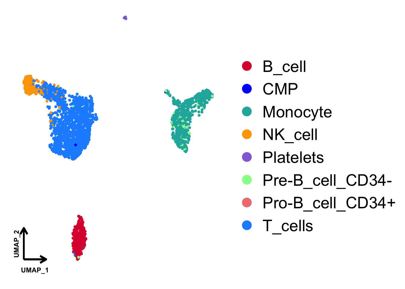

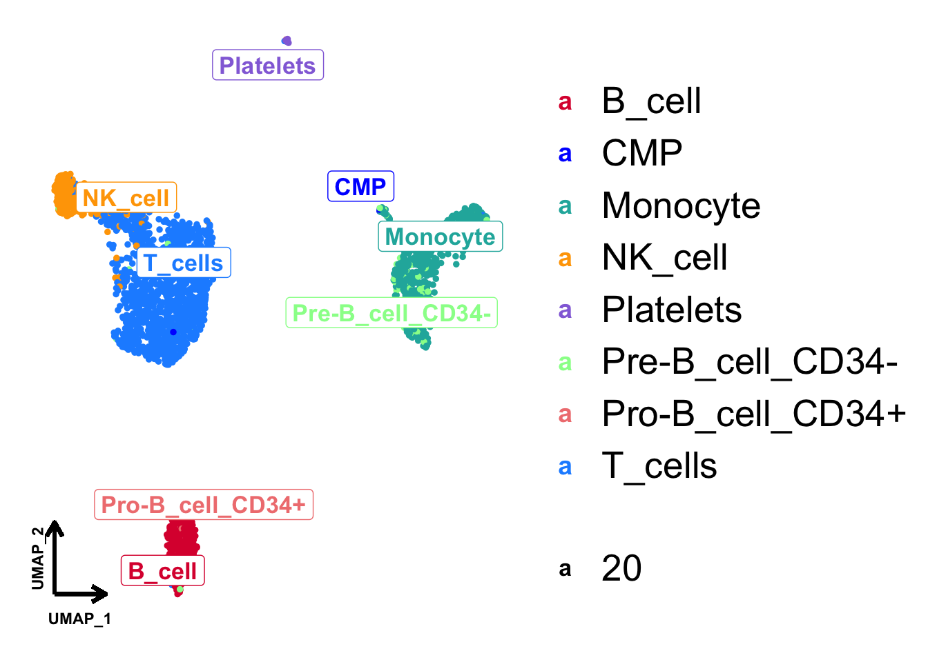
Annotate cell type on UMAP

# Calcualte the median coordinates of each cluster
cell_type_med <- umap |>
  group_by(cell_type) |>
  summarise(UMAP_1 = median(UMAP_1),
    UMAP_2 = median(UMAP_2)
  )
# Annotation
p + geom_label_repel(
    aes(label = cell_type, size = 20), fontface = "bold", data = cell_type_med,
    point.padding = unit(0.5, "lines")
)

FeaturePlot

Default Seurat FeaturePlot

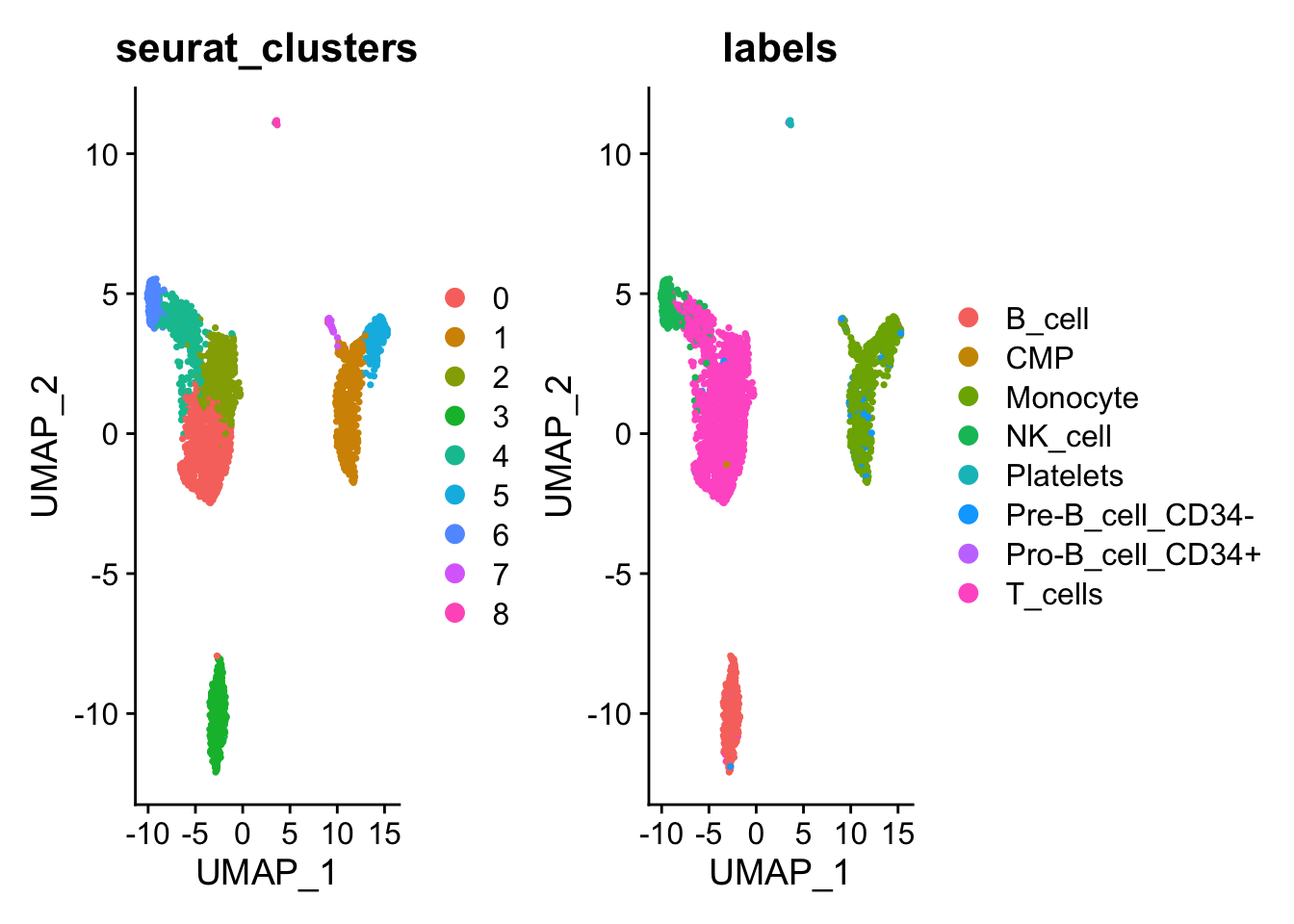
DimPlot(pbmc, label = TRUE)|FeaturePlot(pbmc, features = "CD79A")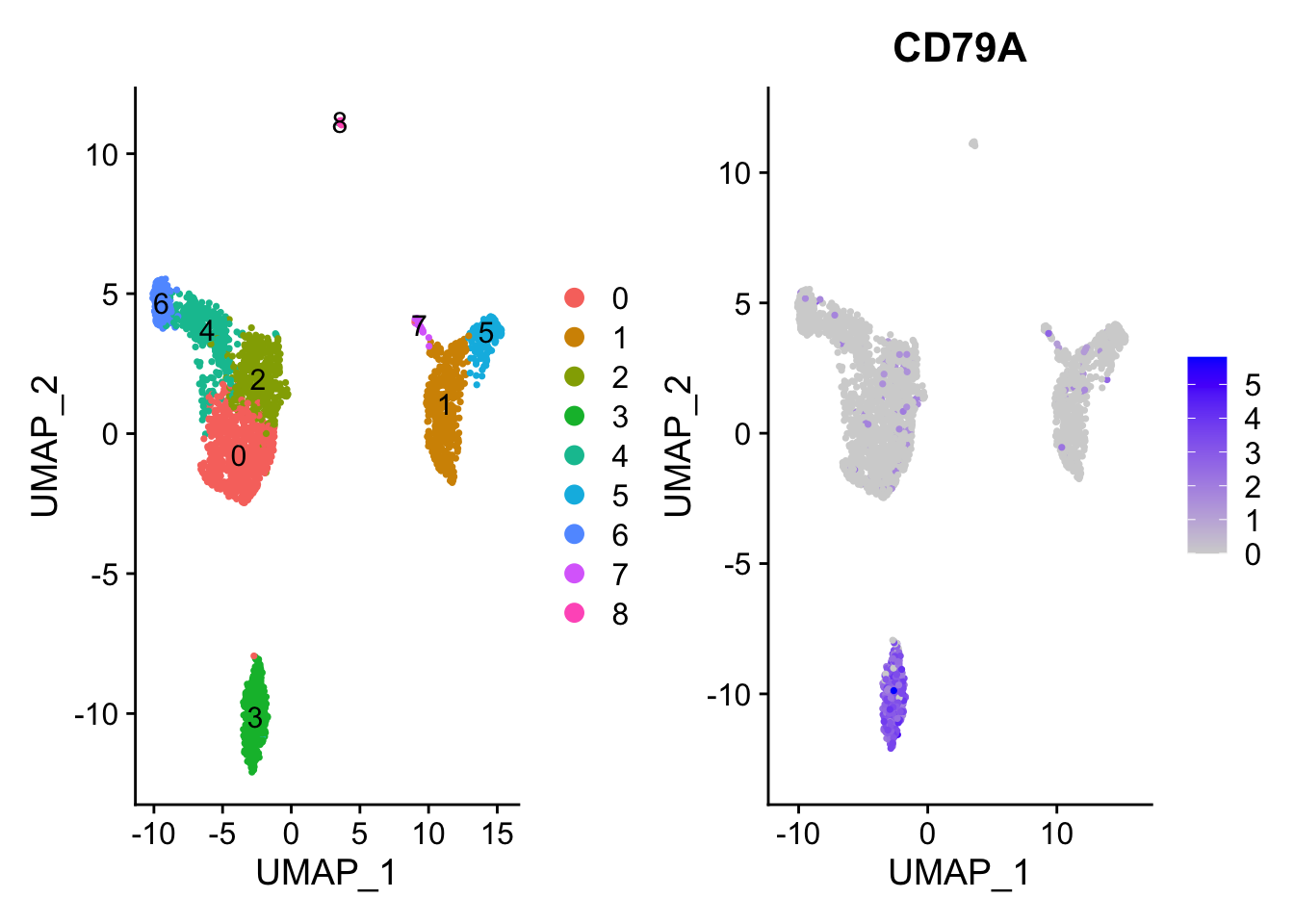

FeaturePlot(pbmc, features = c("CD79A", "CD8A"), blend=TRUE)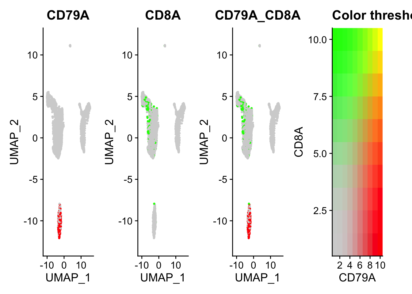

FeaturePlot(pbmc, features = c("CD79A","CD79B"), blend=TRUE)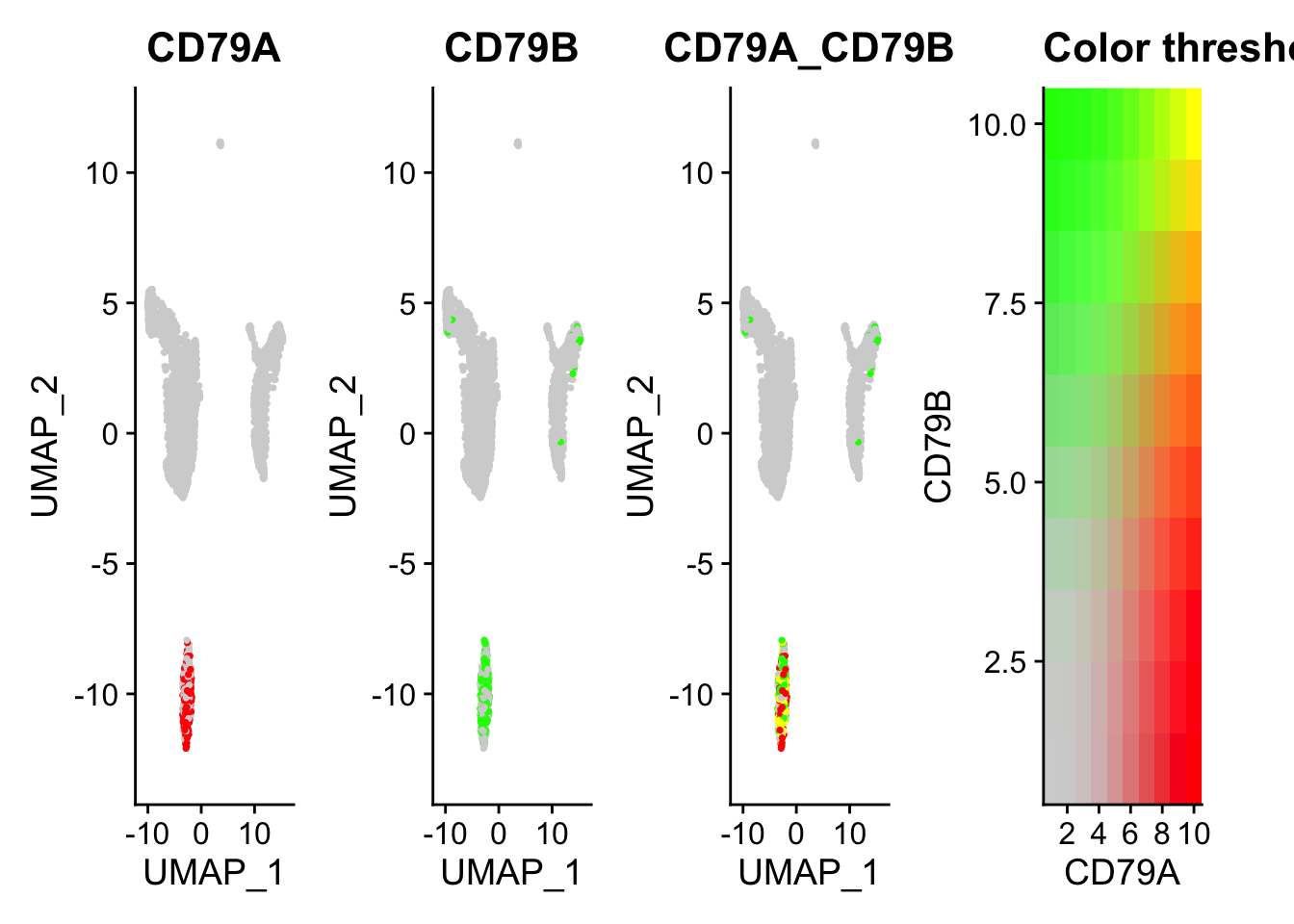

FeaturePlot(pbmc, features = c("CD79A","CD79B", "CD68", "CD163"))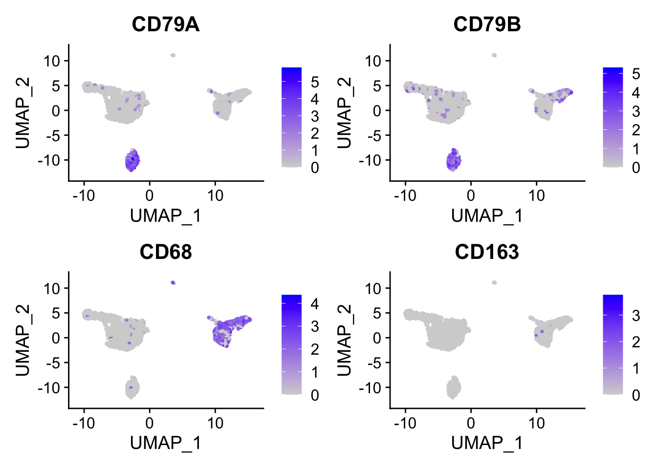

Feature with ggplot2

mydata  <- FetchData(
    pbmc,
    vars = c("rna_CD79A", "rna_CD8A", "rna_CCR7", "UMAP_1", "UMAP_2")
)
head(mydata)
##                  rna_CD79A rna_CD8A rna_CCR7    UMAP_1     UMAP_2
## AAACATACAACCAC-1  0.000000 1.635873 1.635873 -4.577857   1.650203
## AAACATTGAGCTAC-1  1.962726 0.000000 0.000000 -2.813911 -11.897462
## AAACATTGATCAGC-1  0.000000 0.000000 0.000000 -1.684490   3.302480
## AAACCGTGCTTCCG-1  0.000000 0.000000 0.000000 12.694498   2.098798
## AAACCGTGTATGCG-1  0.000000 0.000000 0.000000 -9.829201   3.982013
## AAACGCACTGGTAC-1  0.000000 0.000000 0.000000 -2.908319   1.249230

### Single gene
mydata |>
    ggplot(aes(x = UMAP_1, y = UMAP_2)) +
    geom_point(
        data = mydata, aes(x = UMAP_1, y = UMAP_2,
        color = rna_CD79A), size = 1
    ) +
    ### Increase the transprancy of gray dots
    scale_color_gradient(
        "rna_CD79A", low = alpha("grey", 0.1), 
        high = alpha("red", 1)
    ) +
    ### Density
    stat_density2d(aes(colour=rna_CD79A))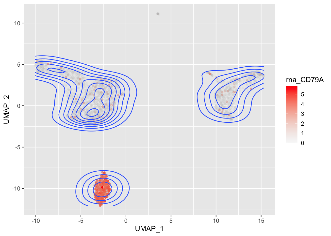

### Multiple genes in feature plot
ggplot(mydata, aes(x = UMAP_1, y = UMAP_2)) +
    geom_point(
        data = mydata, aes(x = UMAP_1, y = UMAP_2, color = rna_CD79A), 
        size = 1
    ) +
    scale_color_gradient(
        "CD79A", low = alpha("grey", 0.1), high = alpha("purple", 1)
    ) +
    new_scale("color") +
    geom_point(
        data = mydata, aes(x = UMAP_1, y = UMAP_2, color = rna_CD8A), 
        size = 1
    ) +
    scale_color_gradient(
        "CD8A", low = alpha("grey", 0.1), high = alpha("red", 1)
    ) +
    new_scale("color") +
    geom_point(
        data = mydata, aes(x = UMAP_1, y = UMAP_2,color = rna_CCR7), 
        size = 1
    ) +
    scale_color_gradient(
        "CCR7", low = alpha("grey", 0.1), high = alpha("green", 1)
    ) +
    theme_bw()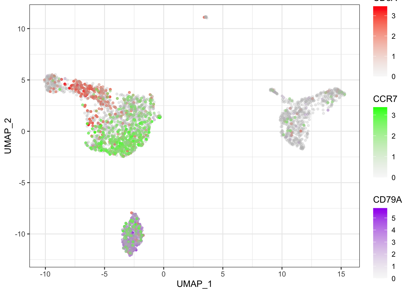

Dotplot

Deafult Dotplot within Seurat

# Find marker genes
# all_markers <- FindAllMarkers(object = sce2)
# save(all_markers,file = here("learn", "2023_scRNA", "all_markers.RData"))

DotPlot(sce2,features = unique(top5$gene) ,assay='RNA')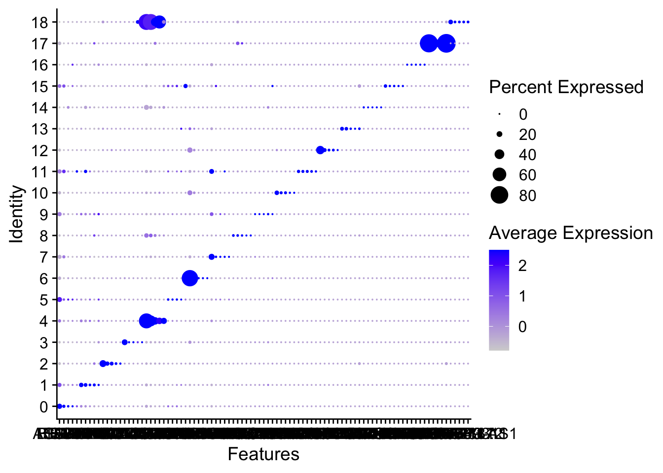

# Optimize colors, size, and direction
p1 <- DotPlot(sce2, features = unique(top5$gene), assay = "RNA") + 
  coord_flip() + 
  labs(x = NULL,y = NULL) + 
  guides(size = guide_legend("Percent Expression"))+
  scale_color_gradientn(colours = c("#330066", "#336699", "#66CC66", "#FFCC33")) +
  theme(
    panel.grid = element_blank(), 
    axis.text.x = element_text(angle = 45, hjust = 0.5,vjust = 0.5)
  )
## Scale for colour is already present.
## Adding another scale for colour, which will replace the existing scale.
p1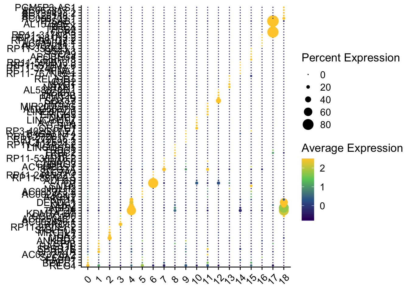

Dotplot with Complexheatmap

We can refer to details from here for detailed parameters customization.

# Retrieve data
df <- p1$data
head(df)
##               avg.exp   pct.exp features.plot id avg.exp.scaled
## REG4       7.70481043 17.174382          REG4  0       2.500000
## BPIFB1     0.30669602  6.860158        BPIFB1  0       2.500000
## FABP1      0.29179596  3.118254         FABP1  0       2.500000
## SLC9A4     0.01901309  1.751019        SLC9A4  0       2.500000
## AC073218.2 0.03103152  1.655073    AC073218.2  0       1.137072
## SPRR1A     0.07460096  3.837851        SPRR1A  0       0.208155

# The matrix for the scaled expression 
exp_mat <-df |> 
  select(-pct.exp, -avg.exp) |>  
  pivot_wider(names_from = id, values_from = avg.exp.scaled) |> 
  as.data.frame()
row.names(exp_mat) <- exp_mat$features.plot
exp_mat <- exp_mat[, -1] |> as.matrix()
head(exp_mat, 2)
##          0          1          2          3          4        5          6
## REG4   2.5  1.0681259 -0.6492553 -0.6766277  0.4956595 1.826576 -0.4005466
## BPIFB1 2.5 -0.1015123 -0.4099583 -0.5370206 -0.3309614 1.039651 -0.6032213
##                 7          8          9         10        11         12
## REG4   -0.3648312 -0.6411552  0.3682808 -0.4876358 0.3408992 -0.6358072
## BPIFB1  0.4017002 -0.5414065 -0.2597756 -0.5685453 1.6007798 -0.6318396
##                13         14        15         16         17         18
## REG4   -0.7044399 -0.7832735 0.5617191 -0.7888883 -0.5395693 -0.7888883
## BPIFB1 -0.6318396 -0.6318396 1.1110916 -0.6318396 -0.6318396 -0.6318396

## The matrix for the percentage of cells express a gene
percent_mat <- df |> 
  select(-avg.exp, -avg.exp.scaled) |>  
  pivot_wider(names_from = id, values_from = pct.exp) |> 
  as.data.frame()
 
row.names(percent_mat) <- percent_mat$features.plot  
percent_mat <- percent_mat[, -1] |> as.matrix()
head(percent_mat, 2)
##                0         1        2         3        4         5         6
## REG4   17.174382 11.642157 5.015480 3.2281731 7.209302 16.111851 7.9301075
## BPIFB1  6.860158  2.389706 1.114551 0.7336757 2.015504  3.062583 0.2688172
##                7         8         9        10        11       12       13 14
## REG4   11.367673 2.5782689 12.406948 7.1090047 12.244898 5.797101 2.380952  1
## BPIFB1  6.571936 0.3683241  1.736973 0.4739336  8.843537 0.000000 0.000000  0
##              15 16       17 18
## REG4   9.278351  0 8.571429  0
## BPIFB1 7.216495  0 0.000000  0

# Complexheatmap
## any value that is greater than 2 will be mapped to yellow
col_fun <-  circlize::colorRamp2(c(-1, 0, 2), viridis(20)[c(1,10, 20)])
cell_fun <- function(j, i, x, y, w, h, fill) {
    grid.rect(x = x, y = y, width = w, height = h,
        gp = gpar(col = NA, fill = NA))
    grid.circle(x = x, y = y, r = percent_mat[i, j] / 100 * min(unit.c(w, h)),
        gp = gpar(fill = col_fun(exp_mat[i, j]), col = NA))
}

# also do a kmeans clustering for the genes with k = 4
Heatmap(
    exp_mat,
    heatmap_legend_param = list(title = "Average Expression"),
    column_title = "clustered dotplot",
    col = col_fun,
    rect_gp = gpar(type = "none"),
    cell_fun = cell_fun,
    row_names_gp = gpar(fontsize = 3),
    # row_km = 4,
    border = "black"
)

# Annotate celltype
colnames(exp_mat)
cluster_anno <- c("Epi", "Myeloid", "Fibroblast", "T", "Endo", "un")

column_ha <- HeatmapAnnotation(
    cluster_anno = cluster_anno,
    col = list(cluster_anno = setNames(brewer.pal(6, "Paired"), unique(cluster_anno))
    ),
    na_col = "grey"
)

Heatmap(
    exp_mat,
    heatmap_legend_param = list(title = "Average Expression"),
    column_title = "clustered dotplot",
    col = col_fun,
    rect_gp = gpar(type = "none"),
    cell_fun = cell_fun,
    row_names_gp = gpar(fontsize = 5),
    # row_km = 4,
    border = "black",
    top_annotation = column_ha
)

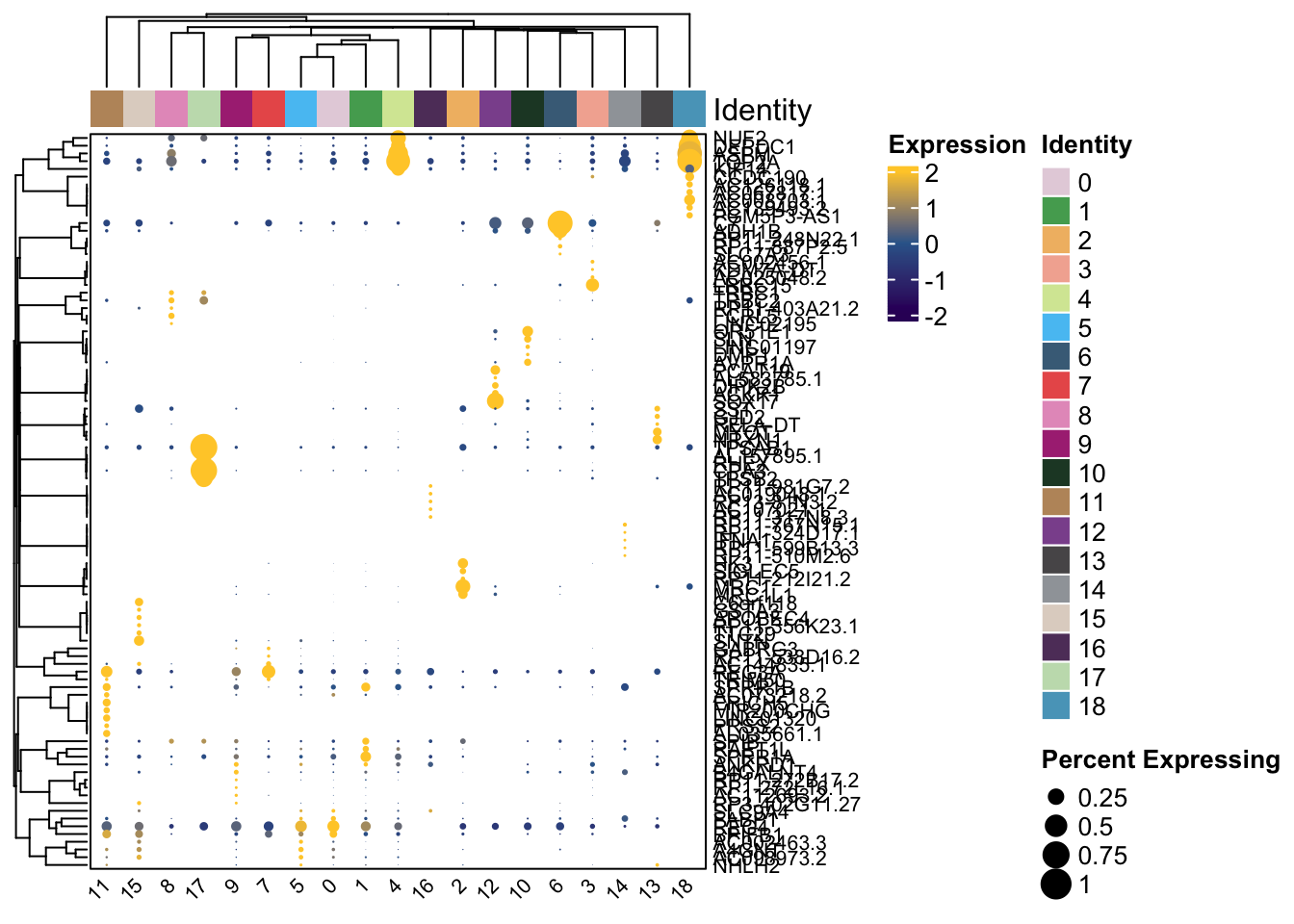
# Add legend
layer_fun <- function(j, i, x, y, w, h, fill) {
    grid.rect(
        x = x, y = y, width = w, height = h, gp = gpar(col = NA, fill = NA)
    )
    grid.circle(
        x = x, y = y, r = pindex(percent_mat, i, j) / 100 * unit(2, "mm"),
        gp = gpar(fill = col_fun(pindex(exp_mat, i, j)), col = NA)
    )
}

lgd_list = list(
    Legend(
        labels = c(0, 0.25, 0.5, 0.75, 1), title = "Percent Expressed",
        graphics = list(
            function(x, y, w, h) grid.circle(x = x, y = y, r = 0 * unit(2, "mm"),
                gp = gpar(fill = "black")),
            function(x, y, w, h) grid.circle(x = x, y = y, r = 0.25 * unit(2, "mm"),
                gp = gpar(fill = "black")),
            function(x, y, w, h) grid.circle(x = x, y = y, r = 0.5 * unit(2, "mm"),
                gp = gpar(fill = "black")),
            function(x, y, w, h) grid.circle(x = x, y = y, r = 0.75 * unit(2, "mm"),
                gp = gpar(fill = "black")),
            function(x, y, w, h) grid.circle(x = x, y = y, r = 1 * unit(2, "mm"),
                gp = gpar(fill = "black"))
        )
    )
)

hp <- Heatmap(
    exp_mat,
    heatmap_legend_param = list(title = "expression"),
    column_title = "clustered dotplot",
    col = col_fun,
    rect_gp = gpar(type = "none"),
    layer_fun = layer_fun,
    row_names_gp = gpar(fontsize = 5),
    # row_km = 4,
    border = "black",
    top_annotation = column_ha
)

draw(hp, annotation_legend_list = lgd_list)

Dotplot with scCustomize

Clustered_DotPlot(seurat_object = sce2, features = unique(top5$gene))

## [[1]]

## 
## [[2]]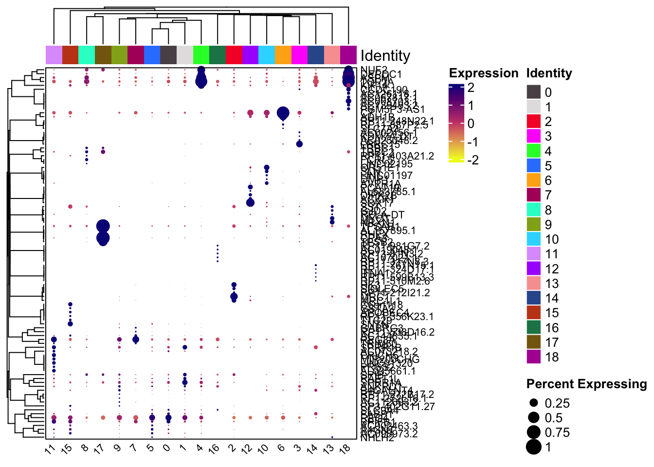


my36colors <- c(
    '#E5D2DD', '#53A85F', '#F1BB72', '#F3B1A0', '#D6E7A3', '#57C3F3', '#476D87',
    '#E95C59', '#E59CC4', '#AB3282', '#23452F', '#BD956A', '#8C549C', '#585658',
    '#9FA3A8', '#E0D4CA', '#5F3D69', '#C5DEBA', '#58A4C3', '#E4C755', '#F7F398',
    '#AA9A59', '#E63863', '#E39A35', '#C1E6F3', '#6778AE', '#91D0BE', '#B53E2B',
    '#712820', '#DCC1DD', '#CCE0F5', '#CCC9E6', '#625D9E', '#68A180', '#3A6963',
    '#968175'
)

Clustered_DotPlot(
    seurat_object = sce2,
    colors_use_exp = c('#330066', '#336699', '#66CC66', '#FFCC33'),
    colors_use_idents = my36colors,
    features = unique(top5$gene)
)

## [[1]]

## 
## [[2]]

DoHeatmap

Deafult DoHeatmap with Seurat

DoHeatmap(sce2, top5$gene)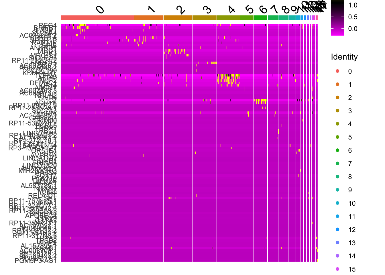

# Customize label and color
DoHeatmap(
    sce2,
    label = F, # remove label
    features = as.character(unique(top5$gene)),
    group.by = "celltype",
    assay = "RNA",
    group.colors = c(
        "#C77CFF", "#7CAE00", "#00BFC4", "#F8766D", "#AB82FF", "#90EE90",
        "#00CD00", "#008B8B", "#FFA500"
    ) # Group color
) +
    scale_fill_gradientn(
        colors = c("navy", "white", "firebrick3")
    ) # heatmap color

Complexheatmap or pheatmap

# Retrieve matix
# mat <- GetAssayData(pbmc,slot = "scale.data")

dittoSeq

# BiocManager::install("dittoSeq")

dittoHeatmap(sce2, top5$gene,
             annot.by = c("celltype", "sample","AUCell"))

scillus

# devtools::install_github("xmc811/Scillus", ref = "development")
# Use same colors of umap  
my36colors <-c(
  '#E5D2DD', '#53A85F', '#F1BB72', '#F3B1A0', '#D6E7A3', '#57C3F3', '#476D87',
  '#E95C59', '#E59CC4', '#AB3282', '#23452F', '#BD956A', '#8C549C', '#585658',
  '#9FA3A8', '#E0D4CA', '#5F3D69', '#C5DEBA', '#58A4C3', '#E4C755', '#F7F398',
  '#AA9A59', '#E63863', '#E39A35', '#C1E6F3', '#6778AE', '#91D0BE', '#B53E2B',
  '#712820', '#DCC1DD', '#CCE0F5',  '#CCC9E6', '#625D9E', '#68A180', '#3A6963',
  '#968175'
)

plot_heatmap(dataset = sce2, 
             markers = top5$gene,
             sort_var = c("celltype","sample"),
             anno_var = c("celltype","sample","percent.mt","AUCell"),
             anno_colors = list(
                "Set2",  # RColorBrewer palette
                my36colors,  # color vecto
                "Reds",
                "Greens")
)

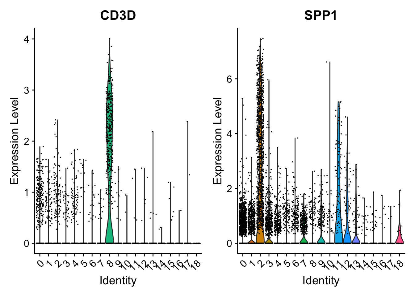
VlnPlot

Default Seurat VlnPlot

# Few marker
VlnPlot(sce2, features = c("CD3D","SPP1"))


# All marker genes
# VlnPlot(sce2, features = top5$gene)

Stacked Vlnplot

a <- VlnPlot(sce2, features = top5$gene, stack = TRUE, sort = TRUE) +
  theme(legend.position = "none") + ggtitle("Identity on y-axis")

# Flip
b <- VlnPlot(sce2, features = top5$gene, stack = TRUE, sort = TRUE, flip = TRUE) +
  theme(legend.position = "none") + ggtitle("Identity on x-axis")

a + b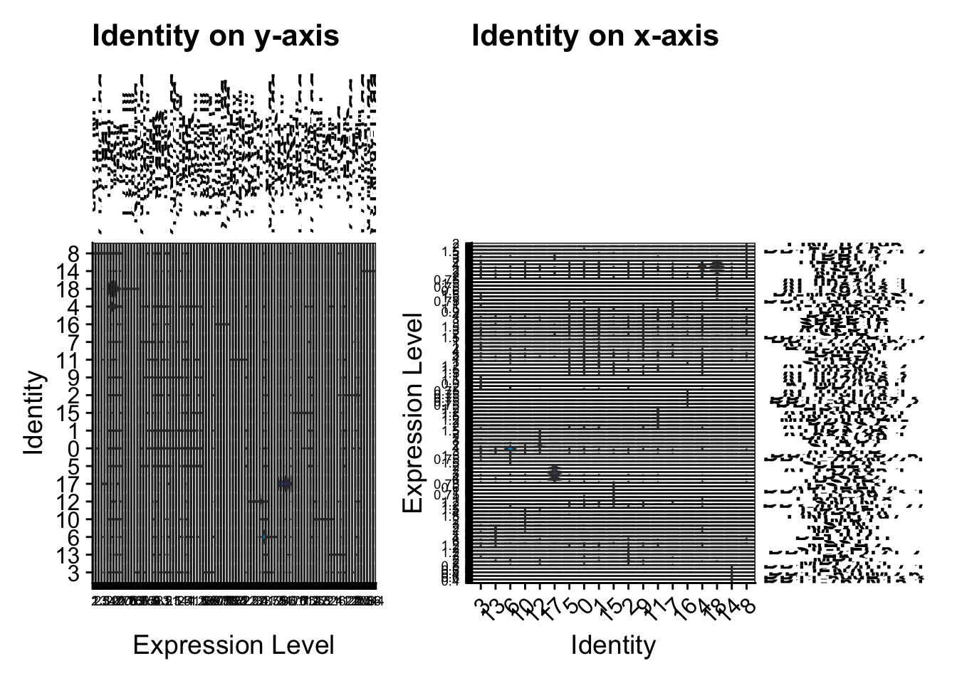

# Optimize colors, size and direction
my36colors <- c(
    '#E5D2DD', '#53A85F', '#F1BB72', '#F3B1A0', '#D6E7A3', '#57C3F3', '#476D87',
    '#E95C59', '#E59CC4', '#AB3282', '#23452F', '#BD956A', '#8C549C', '#585658',
    '#9FA3A8', '#E0D4CA', '#5F3D69', '#C5DEBA', '#58A4C3', '#E4C755', '#F7F398',
    '#AA9A59', '#E63863', '#E39A35', '#C1E6F3', '#6778AE', '#91D0BE', '#B53E2B',
    '#712820', '#DCC1DD', '#CCE0F5', '#CCC9E6', '#625D9E', '#68A180', '#3A6963',
    '#968175'
)

VlnPlot(
    sce2, 
    features = top_marker$gene,
    stack = TRUE,
    sort = TRUE,
    cols = my36colors,
    split.by = "celltype", # color for each cluster
    flip = TRUE
  ) +
    theme(legend.position = "none") +
    ggtitle("Identity on x-axis")

VlnPlot with ggplot2

vln.dat  <- FetchData(sce2, c(top_marker$gene,"celltype","seurat_clusters"))

vln.dat$Cell <- rownames(vln.dat)
vln.dat.melt <- reshape2::melt(vln.dat, id.vars = c("Cell","seurat_clusters"), 
                               measure.vars = top_marker$gene,
                               variable.name = "gene", 
                               value.name = "Expr") |>
  group_by(seurat_clusters,gene) |> 
  mutate(fillcolor=mean(Expr))

# Plot 
ggplot(vln.dat.melt, aes(factor(seurat_clusters), Expr, fill = gene)) +
  geom_violin(scale = "width", adjust = 1, trim = TRUE) +
  facet_grid(rows = vars(gene), scales = "free", switch = "y")

# Customize
p1 <- ggplot(vln.dat.melt, aes(gene, Expr, fill = gene)) +
  geom_violin(scale = "width", adjust = 1, trim = TRUE) +
  scale_y_continuous(expand = c(0, 0), position="right", labels = function(x)
    c(rep(x = "", times = length(x)-2), x[length(x) - 1], "")) +
  facet_grid(rows = vars(seurat_clusters), scales = "free", switch = "y") +
  scale_fill_manual(values = my36colors) + 
  theme_cowplot(font_size = 12) +
  theme(legend.position = "none", panel.spacing = unit(0, "lines"),
        plot.title = element_text(hjust = 0.5),
        panel.background = element_rect(fill = NA, color = "black"),
        plot.margin = margin(7, 7, 0, 7, "pt"),
        strip.background = element_blank(),
        strip.text = element_text(face = "bold"),
        strip.text.y.left = element_text(angle = 0),
        axis.title.x = element_blank(),
        axis.ticks.x = element_blank(),
        axis.text.x = element_text(angle = 90, hjust = 1, vjust = 0.5, color = "black")
        ) +
  ggtitle("Feature on x-axis with annotation") + ylab("Expression Level")
p1

p2 <- ggplot(vln.dat.melt, aes(gene, Expr, fill = gene)) +
  geom_violin(scale = "width", adjust = 1, trim = TRUE) +
  scale_y_continuous(expand = c(0, 0), position="right", labels = function(x)
    c(rep(x = "", times = length(x)-2), x[length(x) - 1], "")) +
  facet_grid(rows = vars(seurat_clusters), scales = "free", switch = "y") +
  scale_fill_manual(values = my36colors) + 
  theme_cowplot(font_size = 12) +
  theme(legend.position = "none", panel.spacing = unit(0, "lines"),
        plot.title = element_text(hjust = 0.5),
        panel.background = element_rect(fill = NA, color = "black"),
        plot.margin = margin(7, 7, 0, 7, "pt"),
        strip.background = element_blank(),
        strip.text = element_text(face = "bold"),
        strip.text.y.left = element_text(angle = 0),
        axis.title.x = element_blank(),
        axis.ticks.x = element_blank(),
        axis.text.x = element_blank()
  ) +
  ggtitle("Feature on x-axis with annotation") + ylab("Expression Level")
p2

# Create grouping info
df <- data.frame(x = levels(vln.dat.melt$gene), 
                 group = c("A","A","B","B","B","B","B","C","C","C","D","D","D",
                           "D","D","D","D","D"), 
                 stringsAsFactors = FALSE)
df$x <- factor(df$x, levels = levels(vln.dat.melt$gene))
df$group <- factor(df$group)

levels(df$group) = c("ECM-receptor interaction", "PI3K-Akt signaling pathway", 
                     "MAPK signaling pathway", "Cell adhesion molecules")

color <- c("cyan", "pink", "green", "darkorange")

p3 <- ggplot(df, aes(x = x, y = 1, fill = group)) + geom_tile() + theme_bw(base_size = 12) +
  scale_fill_manual(values = my36colors) + scale_y_continuous(expand = c(0, 0)) +
  guides(fill = guide_legend(direction = "vertical", label.position = "right",
                             title.theme = element_blank(), keyheight = 0.5, nrow = 2)) +
  theme(legend.position = "bottom",
        legend.justification = "left",
        legend.margin = margin(0,0,0,0),
        legend.box.margin = margin(-10,5,0,0),
        panel.spacing = unit(0, "lines"),
        panel.background = element_blank(),
        panel.border = element_blank(),
        plot.background = element_blank(),
        plot.margin = margin(0, 7, 7, 7, "pt"),
        axis.text.x = element_text(angle = 90, hjust = 1, vjust = 0.5, color = "black"),
        axis.title.y = element_blank(),
        axis.ticks.y = element_blank(),
        axis.text.y = element_blank()) + xlab("Feature")
p3

# Use plot_grid to join plots
plot_grid(p2, p3, ncol = 1, rel_heights = c(0.78, 0.22), align = "v", axis = "lr")

Packages

UMAP

Load Seurat object

Default seurat UMAP

UMAP with ggplot2

Annotate cell type on UMAP

FeaturePlot

Default Seurat FeaturePlot

Feature with ggplot2

Dotplot

Deafult Dotplot within Seurat

Dotplot with Complexheatmap

Dotplot with scCustomize

DoHeatmap

Deafult DoHeatmap with Seurat

Complexheatmap or pheatmap

dittoSeq

scillus

VlnPlot

Default Seurat VlnPlot

Stacked Vlnplot

VlnPlot with ggplot2

Reference