
Harmony to integrating cell line datasets from 10X
data(cell_lines)
scaled_pcs <- cell_lines$scaled_pcs
meta_data <- cell_lines$meta_data
### cells cluster by dataset initially
p1 <- do_scatter(scaled_pcs, meta_data, "dataset") +
    labs(title = "Colored by dataset")
p2 <- do_scatter(scaled_pcs, meta_data, "cell_type") +
    labs(title = "Colored by cell type")
### combine plot
cowplot::plot_grid(p1, p2)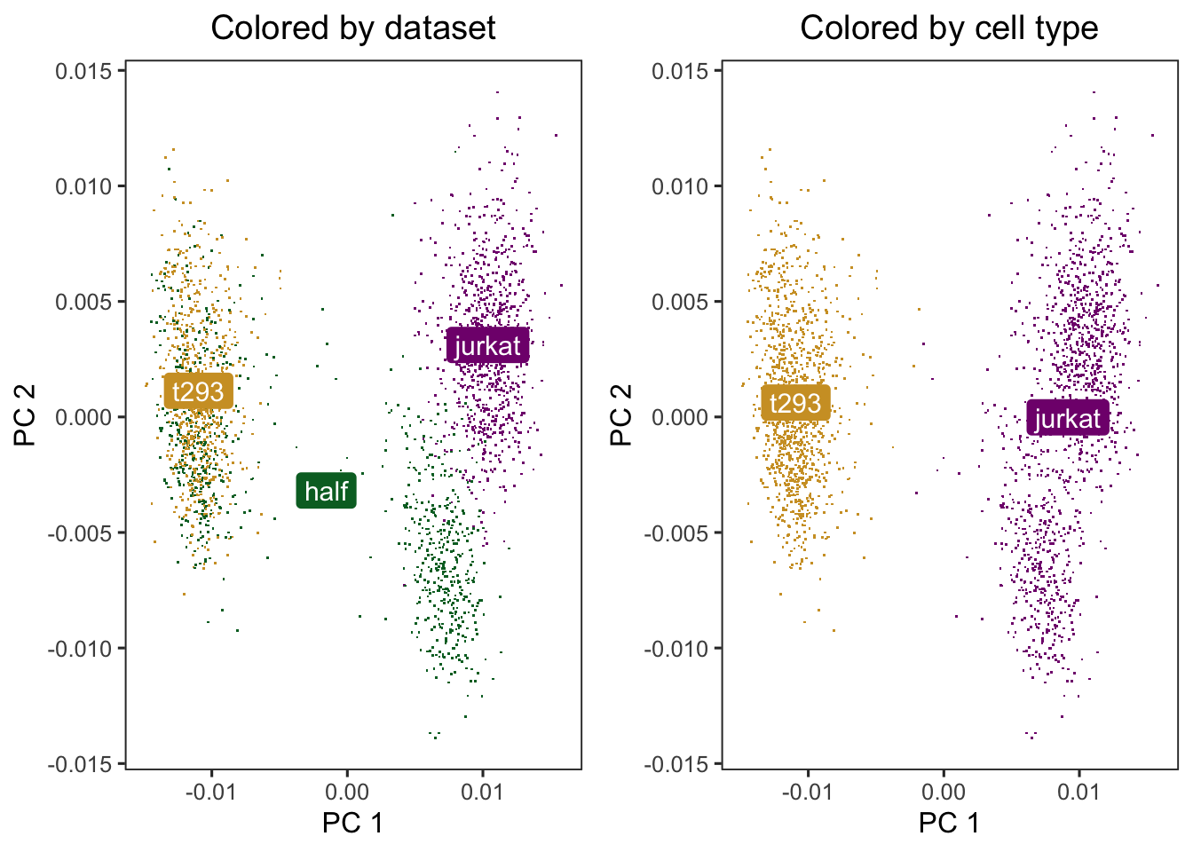
Run harmonoy to remove the influence of dataset-of origin from ceel embeddings. After Harmony, the datasets are now mixed and the cell types are still separate.
harmony_embeddings <- harmony::RunHarmony(
    scaled_pcs, meta_data, "dataset", verbose = FALSE
)
p1 <- do_scatter(harmony_embeddings, meta_data, "dataset") +
labs(title = "Colored by dataset")
p2 <- do_scatter(harmony_embeddings, meta_data, "cell_type") +
    labs(title = "Colored by cell type")
### combine plot
cowplot::plot_grid(p1, p2, nrow = 1)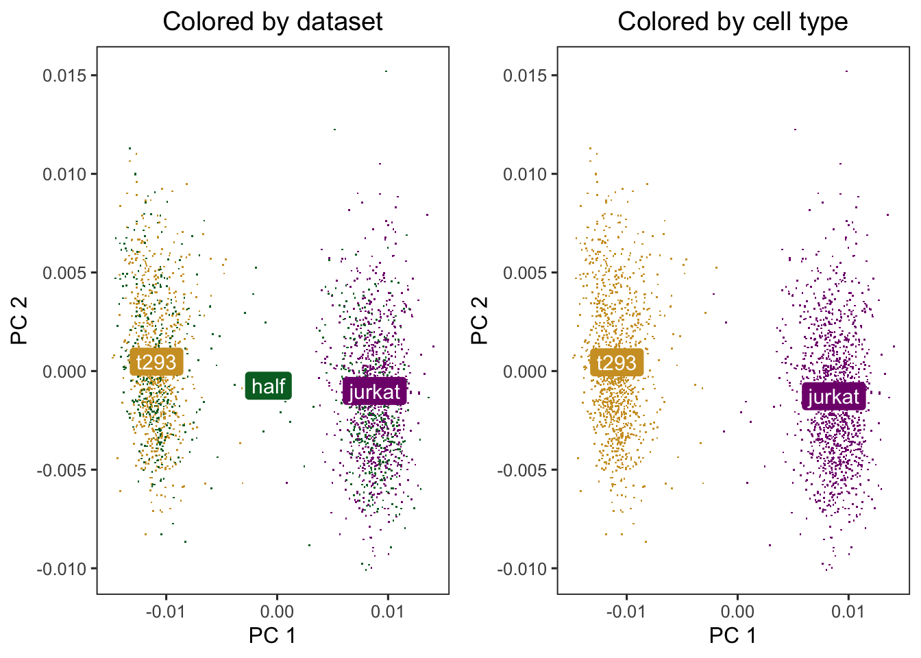
MUDAN
Combine the two datasets into one cell by gene counts matrix and use a meta vector to keep track of which cell belongs to which sample
### combine into one coutns matrix
genes_int <- intersect(rownames(pbmcA), rownames(pbmcB))
cd <- cbind(pbmcA[genes_int, ], pbmcB[genes_int, ])

### meta data
meta <- c(rep("pbmcA", ncol(pbmcA)), rep("pbmcB", ncol(pbmcB)))
names(meta) <- c(colnames(pbmcA), colnames(pbmcB))
meta <- factor(meta)

cd[1:5, 1:2]
meta[1:5]
Given this counts matrix, we can normalize our data, derive principal components, and perform dimensionality reduction using tSNE. However, we see prominent separation by sample due to batch effects.
### CPM normalization
mat <- MUDAN::normalizeCounts(cd, verbose = FALSE)

### variance normalize, identify overdispersed genes
matnorm_info <- MUDAN::normalizeVariance(mat, details = TRUE, verbose = FALSE)

### log transform
matnorm <- log10(matnorm_info$mat + 1)

### 30 PCs on over dispersed genes
pcs <- MUDAN::getPcs(
    matnorm[matnorm_info$ods, ],
    nGenes = length(matnorm_info$ods),
    nPcs = 30,
    verbose = FALSE
)
### TSNE embedding with regular PCS
emb <- Rtsne::Rtsne(
    pcs,
    is_distance = FALSE,
    perplexity = 30,
    num_threads = 1,
    verbose = FALSE
)$Y
rownames(emb) <- rownames(pcs)
### plot
par(mfrow = c(1, 1), mar = rep(2, 4))
MUDAN::plotEmbedding(
    emb, groups = meta, show.legend = TRUE,
    xlab = NA, ylab = NA,
    main = "Regular tSNE Embedding",
    verbose = FALSE
)
Indeed, when we inspect certain cell-type specific marker genes (MS4A1/CD20 for B-cells, CD3E for T-cells, FCGR3A/CD16 for NK cells, macrophages, and monocytes, CD14 for dendritic cells, macrophages, and monocytes), we see that cells are separating by batch rather than by their expected cell-types.
If we were attempt to identify cell-types using clustering analysis at this step, we would identify a number of sample-specific clusters driven by batch effects.
annot_bad <- getComMembership(pcs, k = 30, method = igraph::cluster_louvain)
par(mfrow = c(1, 1), mar = rep(2, 4))
plotEmbedding(
    emb, groups = annot_bad, show.legend = TRUE,
    xlab = NA, ylab = NA,
    main = "Jointly-indentified cell clusters",
    verbose = FALSE
)
### look at cell-type proportion per sample
t(table(annot_bad, meta))/as.numeric(table(meta))
# Look at cell-type proportions per sample
# print(t(table(annot_bad, meta))/as.numeric(table(meta)))Using Harmony with Seurat
### load required data
data("pbmc_stim")

### generate seurat object
pbmc <- CreateSeuratObject(
    counts = cbind(pbmc.stim, pbmc.ctrl),
    project = "PBMC",
    min.cells = 5
)

### separete conditions
pbmc@meta.data$stim <- c(
    rep("STIM", ncol(pbmc.stim)),
    rep("CTRL", ncol(pbmc.ctrl))
)

### generate a union of highly variable genes
pbmc <- pbmc |> Seurat::NormalizeData(verbose = FALSE)

VariableFeatures(pbmc) <- split(row.names(pbmc@meta.data), pbmc@meta.data$stim) %>% lapply(function(cells_use) {
    pbmc[,cells_use] %>%
        FindVariableFeatures(selection.method = "vst", nfeatures = 2000) %>%
        VariableFeatures()
}) %>% unlist %>% unique
## Finding variable features for layer counts
## Finding variable features for layer counts

pbmc <- pbmc |>
    ScaleData(verbose = FALSE) |>
    RunPCA(features = VariableFeatures(pbmc), npcs = 20, verbose = FALSE)
Clear difference between the datasets in the uncorrected PCs
p1 <- DimPlot(object = pbmc, reduction = "pca", pt.size = .1, group.by = "stim")
p2 <- VlnPlot(object = pbmc, features = "PC_1", group.by = "stim", pt.size = .1)
cowplot::plot_grid(p1,p2)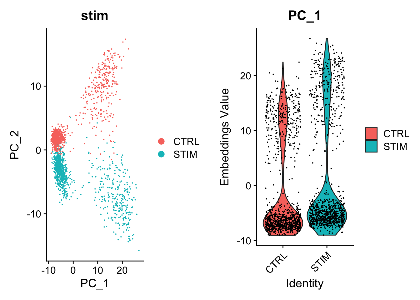
Run Harmony
Harmony works on an existing matrix with cell embeddings and outputs its transformed version with the datasets aligned according to some user-defined experimental conditions.
### run harmony to perform integrated analysis
pbmc <- RunHarmony(pbmc, "stim", plot_convergence = TRUE)
## Transposing data matrix
## Initializing state using k-means centroids initialization
## Harmony 1/10
## Harmony 2/10
## Harmony 3/10
## Harmony 4/10
## Harmony 5/10
## Harmony 6/10
## Harmony 7/10
## Harmony 8/10
## Harmony 9/10
## Harmony converged after 9 iterations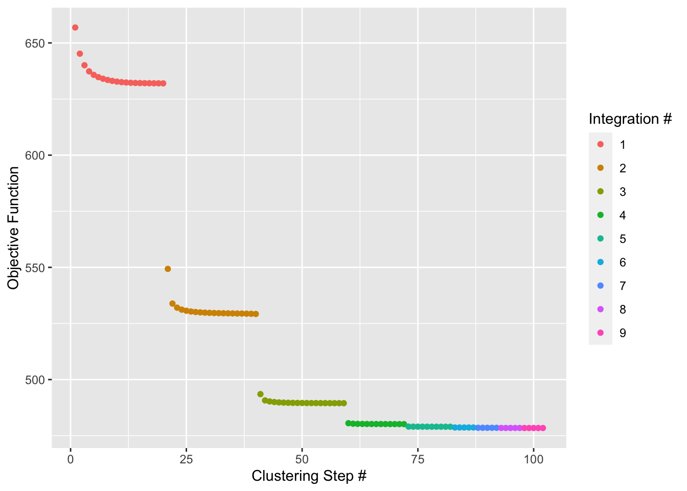
### directly access the new harmony embeddings
harmony_embeddings <- Embeddings(pbmc, "harmony")
harmony_embeddings[1:5, 1:5]
##                  harmony_1   harmony_2   harmony_3 harmony_4    harmony_5
## ATCACTTGCTCGAA-1 -6.472885 -0.03395769 -3.37113988  4.104260  0.001600968
## CCGGAGACTGTGAC-1 -6.901013  1.59104949 -6.36127179  4.635761 -5.605371816
## CAAGCCCTGTTAGC-1 -6.774086 -1.21811545 -6.49162911 -9.135284 -0.197759676
## GAGGTACTAACGGG-1 -7.435499 -0.23169621  0.07052885  2.031633 -2.190562901
## CGCGGATGCCACAA-1 14.686943  4.38600212 -4.49637985  1.595446 -1.448223157

### inspection of the modalities
p1 <- DimPlot(object = pbmc, reduction = "harmony", pt.size = .1, group.by = "stim")
p2 <- VlnPlot(object = pbmc, features = "harmony_1", group.by = "stim", pt.size = .1)
plot_grid(p1,p2)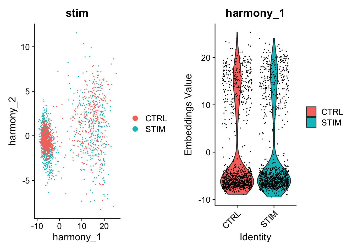
Plot genes correlated with the harmonized PCs
DimHeatmap(object = pbmc, reduction = "harmony", cells = 500, dims = 1:3)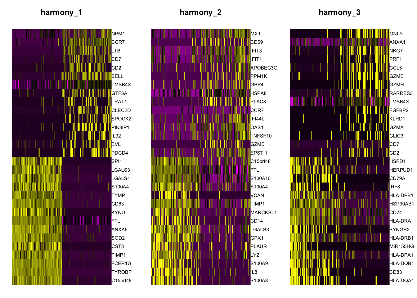
Down stream analysis
pbmc <- pbmc |>
    ### perform clustering using the harmonized vectors of cells
    FindNeighbors(reduction = "harmony", dims = 1:20) |>
    FindClusters(resolution = 0.5) |>
    identity()
## Computing nearest neighbor graph
## Computing SNN
## Modularity Optimizer version 1.3.0 by Ludo Waltman and Nees Jan van Eck
##
## Number of nodes: 2000
## Number of edges: 85805
##
## Running Louvain algorithm...
## Maximum modularity in 10 random starts: 0.8883
## Number of communities: 10
## Elapsed time: 0 seconds
### TSNE
pbmc <- pbmc %>%
    RunTSNE(reduction = "harmony")
p1 <- DimPlot(pbmc, reduction = "tsne", group.by = "stim", pt.size = .1)
p2 <- DimPlot(pbmc, reduction = "tsne", label = TRUE, pt.size = .1)
plot_grid(p1, p2)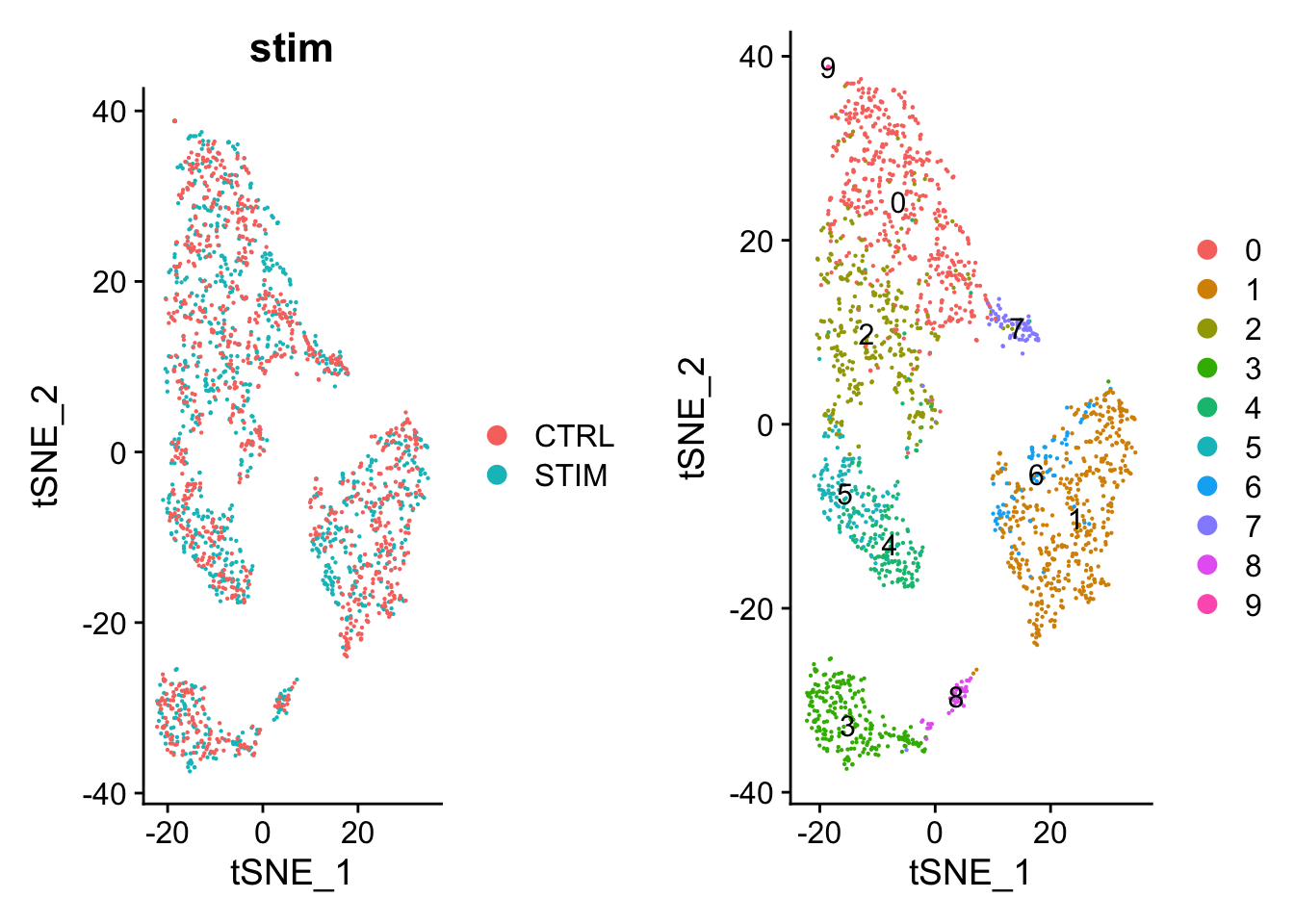
One important observation is to assess that the harmonized data contain biological states of the cells. Therefore by checking the following genes we can see that biological cell states are preserved after harmonization.
FeaturePlot(object = pbmc, features= c("CD3D", "SELL", "CREM", "CD8A", "GNLY", "CD79A", "FCGR3A", "CCL2", "PPBP"),
            min.cutoff = "q9", cols = c("lightgrey", "blue"), pt.size = 0.5)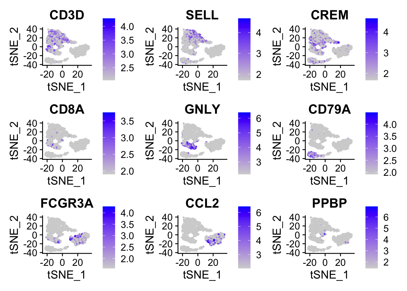
### UMAP
pbmc <- pbmc |>
    RunUMAP(reduction = "harmony", dims = 1:20)
## 20:34:54 UMAP embedding parameters a = 0.9922 b = 1.112
## Found more than one class "dist" in cache; using the first, from namespace 'BiocGenerics'
## Also defined by 'spam'
## 20:34:54 Read 2000 rows and found 20 numeric columns
## 20:34:54 Using Annoy for neighbor search, n_neighbors = 30
## Found more than one class "dist" in cache; using the first, from namespace 'BiocGenerics'
## Also defined by 'spam'
## 20:34:54 Building Annoy index with metric = cosine, n_trees = 50
## 0%   10   20   30   40   50   60   70   80   90   100%
## [----|----|----|----|----|----|----|----|----|----|
## **************************************************|
## 20:34:54 Writing NN index file to temp file /var/folders/2c/9q3pg2295195bp3gnrgbzrg40000gn/T//RtmpBhrb7C/file51ff59f4665b
## 20:34:54 Searching Annoy index using 1 thread, search_k = 3000
## 20:34:54 Annoy recall = 100%
## 20:34:54 Commencing smooth kNN distance calibration using 1 thread with target n_neighbors = 30
## 20:34:55 Initializing from normalized Laplacian + noise (using RSpectra)
## 20:34:55 Commencing optimization for 500 epochs, with 83254 positive edges
## 20:34:57 Optimization finished
p1 <- DimPlot(pbmc, reduction = "umap", group.by = "stim", pt.size = .1, split.by = 'stim')
### identify shared cell types with clustering analysis
p2 <- DimPlot(pbmc, reduction = "umap", label = TRUE, pt.size = .1)
plot_grid(p1, p2)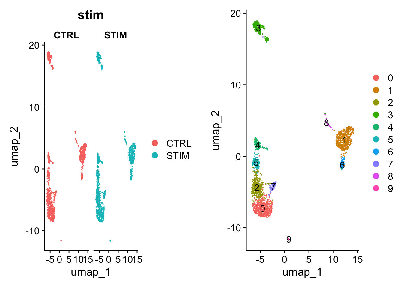
Reference
Session info
sessionInfo()
## R version 4.3.1 (2023-06-16)
## Platform: aarch64-apple-darwin20 (64-bit)
## Running under: macOS Sonoma 14.2
##
## Matrix products: default
## BLAS:   /Library/Frameworks/R.framework/Versions/4.3-arm64/Resources/lib/libRblas.0.dylib
## LAPACK: /Library/Frameworks/R.framework/Versions/4.3-arm64/Resources/lib/libRlapack.dylib;  LAPACK version 3.11.0
##
## locale:
## [1] en_US.UTF-8/en_US.UTF-8/en_US.UTF-8/C/en_US.UTF-8/en_US.UTF-8
##
## time zone: Asia/Singapore
## tzcode source: internal
##
## attached base packages:
## [1] stats     graphics  grDevices utils     datasets  methods   base
##
## other attached packages:
##  [1] cowplot_1.1.1      here_1.0.1         lubridate_1.9.3    forcats_1.0.0
##  [5] stringr_1.5.1      dplyr_1.1.4        purrr_1.0.2        readr_2.1.4
##  [9] tidyr_1.3.0        tibble_3.2.1       ggplot2_3.4.4      tidyverse_2.0.0
## [13] Seurat_5.0.1       SeuratObject_5.0.1 sp_2.1-2           MUDAN_0.1.0
## [17] Matrix_1.6-3       harmony_1.1.0      Rcpp_1.0.11
##
## loaded via a namespace (and not attached):
##   [1] RcppAnnoy_0.0.21        splines_4.3.1           later_1.3.1
##   [4] bitops_1.0-7            polyclip_1.10-6         XML_3.99-0.15
##   [7] fastDummies_1.7.3       lifecycle_1.0.4         rprojroot_2.0.4
##  [10] edgeR_4.0.1             globals_0.16.2          lattice_0.22-5
##  [13] MASS_7.3-60             magrittr_2.0.3          limma_3.58.1
##  [16] plotly_4.10.3           rmarkdown_2.25          yaml_2.3.7
##  [19] httpuv_1.6.12           sctransform_0.4.1       spam_2.10-0
##  [22] spatstat.sparse_3.0-3   reticulate_1.34.0       pbapply_1.7-2
##  [25] DBI_1.1.3               RColorBrewer_1.1-3      abind_1.4-5
##  [28] zlibbioc_1.48.0         Rtsne_0.16              BiocGenerics_0.48.1
##  [31] RCurl_1.98-1.13         sva_3.50.0              GenomeInfoDbData_1.2.11
##  [34] IRanges_2.36.0          S4Vectors_0.40.2        ggrepel_0.9.4
##  [37] irlba_2.3.5.1           listenv_0.9.0           spatstat.utils_3.0-4
##  [40] genefilter_1.84.0       goftest_1.2-3           RSpectra_0.16-1
##  [43] spatstat.random_3.2-2   annotate_1.80.0         fitdistrplus_1.1-11
##  [46] parallelly_1.36.0       leiden_0.4.3.1          codetools_0.2-19
##  [49] tidyselect_1.2.0        farver_2.1.1            matrixStats_1.1.0
##  [52] stats4_4.3.1            spatstat.explore_3.2-5  jsonlite_1.8.7
##  [55] ellipsis_0.3.2          progressr_0.14.0        ggridges_0.5.4
##  [58] survival_3.5-7          tools_4.3.1             ica_1.0-3
##  [61] glue_1.6.2              gridExtra_2.3           xfun_0.41
##  [64] mgcv_1.9-0              MatrixGenerics_1.14.0   GenomeInfoDb_1.38.0
##  [67] withr_2.5.2             fastmap_1.1.1           fansi_1.0.5
##  [70] digest_0.6.33           timechange_0.2.0        R6_2.5.1
##  [73] mime_0.12               colorspace_2.1-0        scattermore_1.2
##  [76] tensor_1.5              spatstat.data_3.0-3     RSQLite_2.3.3
##  [79] RhpcBLASctl_0.23-42     utf8_1.2.4              generics_0.1.3
##  [82] data.table_1.14.8       httr_1.4.7              htmlwidgets_1.6.3
##  [85] uwot_0.1.16             pkgconfig_2.0.3         gtable_0.3.4
##  [88] blob_1.2.4              lmtest_0.9-40           XVector_0.42.0
##  [91] htmltools_0.5.7         dotCall64_1.1-1         scales_1.3.0
##  [94] Biobase_2.62.0          png_0.1-8               knitr_1.45
##  [97] tzdb_0.4.0              reshape2_1.4.4          nlme_3.1-163
## [100] cachem_1.0.8            zoo_1.8-12              KernSmooth_2.23-22
## [103] vipor_0.4.5             parallel_4.3.1          miniUI_0.1.1.1
## [106] AnnotationDbi_1.64.1    ggrastr_1.0.2           pillar_1.9.0
## [109] grid_4.3.1              vctrs_0.6.5             RANN_2.6.1
## [112] promises_1.2.1          xtable_1.8-4            cluster_2.1.4
## [115] beeswarm_0.4.0          evaluate_0.23           cli_3.6.1
## [118] locfit_1.5-9.8          compiler_4.3.1          rlang_1.1.2
## [121] crayon_1.5.2            future.apply_1.11.0     labeling_0.4.3
## [124] ggbeeswarm_0.7.2        plyr_1.8.9              stringi_1.8.2
## [127] viridisLite_0.4.2       deldir_2.0-2            BiocParallel_1.36.0
## [130] munsell_0.5.0           Biostrings_2.70.1       lazyeval_0.2.2
## [133] spatstat.geom_3.2-7     RcppHNSW_0.5.0          hms_1.1.3
## [136] patchwork_1.1.3         bit64_4.0.5             future_1.33.0
## [139] KEGGREST_1.42.0         statmod_1.5.0           shiny_1.8.0
## [142] ROCR_1.0-11             igraph_1.5.1            memoise_2.0.1
## [145] bit_4.0.5