### Load packages
pacman::p_load(ggplot2, dplyr, ggpubr, ggbeeswarm, readxl, rstatix, here)

### Import dataset
dataset <- read_excel(here("learn", "Superplots_R_script", "data.xlsx"))

## Defines a colorblind-friendly palette
cbPalette <- c("#999999", "#E69F00", "#56B4E9", "#009E73", "#F0E442", "#0072B2", "#D55E00", "#CC79A7")

## Order the variables on x-axis
dataset$variable <- factor(dataset$variable, levels = c("Before", "After"))

## Calculate averages of each replicate
replicate_mean <- dataset |> group_by(variable, replicate) |>
    summarise_at(vars(value), mean, na.rm =  TRUE) |>
    ungroup()
### view the data
replicate_mean
## # A tibble: 6 × 3
##   variable replicate value
##   <fct>        <dbl> <dbl>
## 1 Before           1  20.8
## 2 Before           2  23
## 3 Before           3  20.2
## 4 After            1  51.4
## 5 After            2  41.2
## 6 After            3  55.8

## Perform t-test of variable 1 and 2
# t_test <- t.test(
#     x = replicate_mean$value[1:3],
#     y = replicate_mean$value[4:6],
#     alternative = "two.sided",
#     var.equal =  TRUE
# )
### Retrieve the p-value for the t-test of variable 1 and 2
# pvalue <- t_test["p.value"]

pvalue <- replicate_mean |>
    t_test(value ~ variable) |>
    add_significance(p.col = "p")

## Calculate total average
total_mean <- replicate_mean |>
    group_by(variable) |>
summarise_at(vars(value), mean, na.rm = TRUE)The code is adapted from here
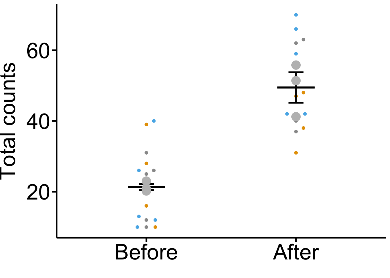
## Plots Superplot based on biological repicate averags
ggplot(dataset, aes(x = variable, y = value, color = factor(replicate))) +
    ### Add individual data points
    geom_beeswarm(cex = 3) +
    #### "cex" can be used to spread the data points if the averages are close together

    ### Add mean values as bars
    stat_summary(data = total_mean, fun = mean, fun.min = mean,
    fun.max = mean, geom = "crossbar", width = 0.25, color = "black") +

    ### Add error bars
    stat_summary(data = replicate_mean, fun.data = mean_se,
    geom = "errorbar", width = 0.1, color = "black", linewidth = 1) +

    ### Add color palette
    scale_color_manual(values = cbPalette) +

    ### Add replicate averages as points
    geom_beeswarm(data = replicate_mean, size = 5, color = "gray") +

    ### Add pvalue
    # stat_pvalue_manual(
    #     pvalue, y.postion = 80, step.increase = 0.1,
    #     label = "p = {p.signif}"
    # ) +

    ### Cosmetics and labeling
    labs(x = "", y = "Total counts") +
    theme_bw() +
    theme(
        axis.line = element_line(size = 1, colour = "black"),
        legend.position = "none",
        axis.title.y = element_text(family="Arial", size=28, color = "black", vjust = 2),
        axis.text = element_text(family="Arial", size = 28, color = "black"),
        axis.ticks = element_line(size = 1, color = "black"),
        axis.ticks.length = unit(2, "mm"),
        panel.grid.major = element_blank(),
        panel.grid.minor = element_blank(),
        panel.background = element_blank(),
        panel.border = element_blank()
    )