Guorui Zhong - Analyze Omics data using [structToolbox]

Packages

pacman::p_load(
    ### BiocManager packages
    structToolbox,
    pmp,
    ropls,
    BiocFileCache,
    ### CRAN packages
    cowplot,
    openxlsx,
    ggplot2, 
    gridExtra
)

### use the BiocFileCache
# bfc <- BiocFileCache(ask = FALSE)

Dataset

### iris dataset
D <- iris_DatasetExperiment()
D$sample_meta$class <- D$sample_meta$Species
D
## A "DatasetExperiment" object
## ----------------------------
## name:          Fisher's Iris dataset
## description:   This famous (Fisher's or Anderson's) iris data set gives the measurements in centimeters of
##                  the variables sepal length and width and petal length and width,
##                  respectively, for 50 flowers from each of 3 species of iris. The species are
##                  Iris setosa, versicolor, and virginica.
## data:          150 rows x 4 columns
## sample_meta:   150 rows x 2 columns
## variable_meta: 4 rows x 1 columns
head(D$data[, 1:4])
##   Sepal.Length Sepal.Width Petal.Length Petal.Width
## 1          5.1         3.5          1.4         0.2
## 2          4.9         3.0          1.4         0.2
## 3          4.7         3.2          1.3         0.2
## 4          4.6         3.1          1.5         0.2
## 5          5.0         3.6          1.4         0.2
## 6          5.4         3.9          1.7         0.4

Using {struct} model objects

### Statistical models
P = PCA(number_components=15)
P$number_components  <-  5
P$number_components
## [1] 5
### the input for a model can be listed using:
param_ids(P)
## [1] "number_components"
P
## A "PCA" object
## --------------
## name:          Principal Component Analysis (PCA)
## description:   PCA is a multivariate data reduction technique. It summarises the data in a smaller number of
##                  Principal Components that maximise variance.
## input params:  number_components 
## outputs:       scores, loadings, eigenvalues, ssx, correlation, that 
## predicted:     that
## seq_in:        data
### model sequences
M = mean_centre() + PCA(number_components = 4)
M[2]$number_components
## [1] 4
### training/testing models
M = model_train(M, D)
M = model_predict(M,D)
M = model_apply(M,D)
output_ids(M[2])
## [1] "scores"      "loadings"    "eigenvalues" "ssx"         "correlation"
## [6] "that"

### model charts
chart_names(M[2])
## [1] "pca_biplot"           "pca_correlation_plot" "pca_dstat_plot"      
## [4] "pca_loadings_plot"    "pca_scores_plot"      "pca_scree_plot"
### plot PCA scores plot
C = pca_scores_plot(factor_name='class') # colour by class
chart_plot(C,M[2])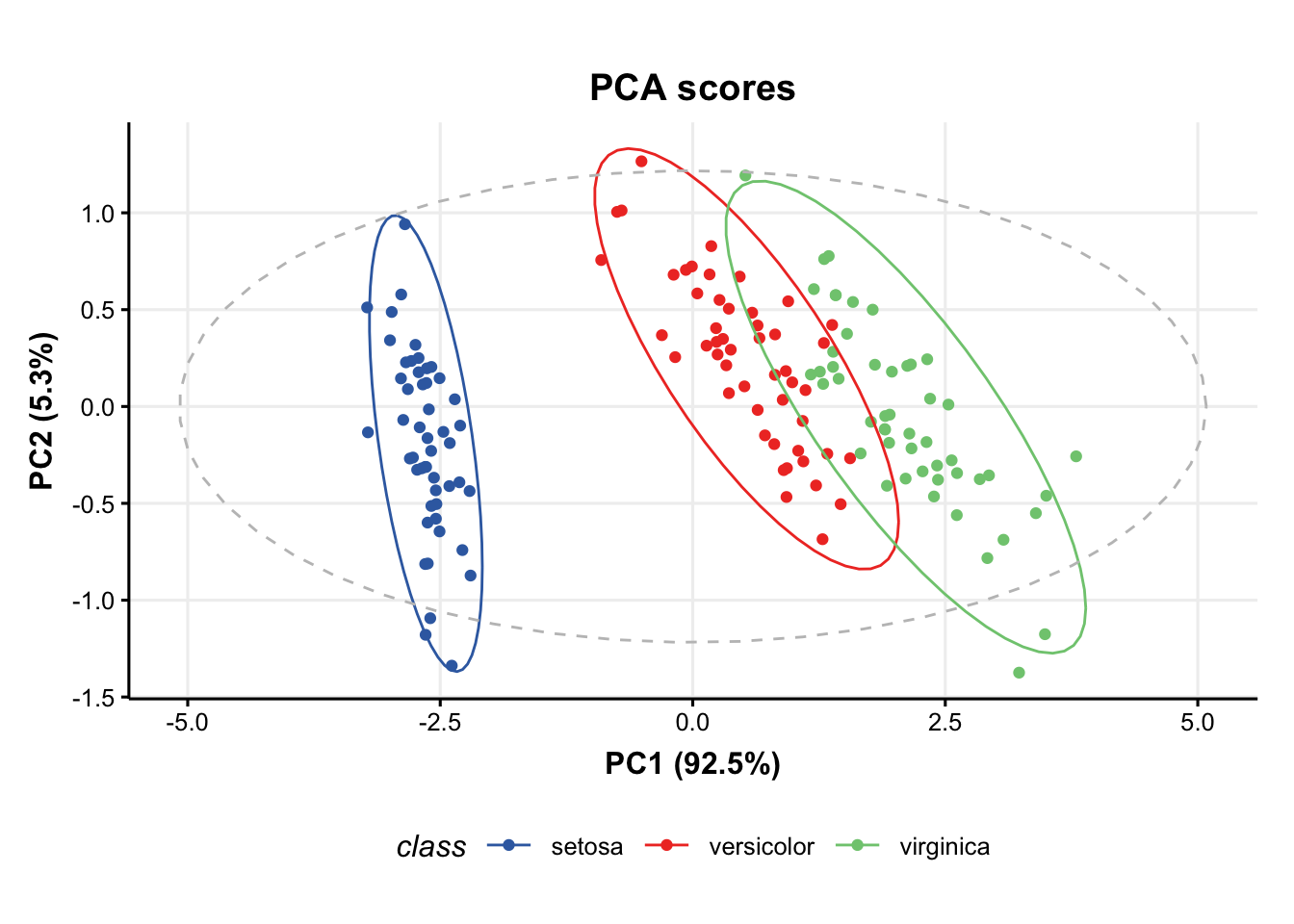


# add petal width to meta data of pca scores
M[2]$scores$sample_meta$example=D$data[,1]
# update plot
C$factor_name='example'
chart_plot(C,M[2])
## Warning: The following aesthetics were dropped during statistical transformation: colour
## ℹ This can happen when ggplot fails to infer the correct grouping structure in
##   the data.
## ℹ Did you forget to specify a `group` aesthetic or to convert a numerical
##   variable into a factor?
## The following aesthetics were dropped during statistical transformation: colour
## ℹ This can happen when ggplot fails to infer the correct grouping structure in
##   the data.
## ℹ Did you forget to specify a `group` aesthetic or to convert a numerical
##   variable into a factor?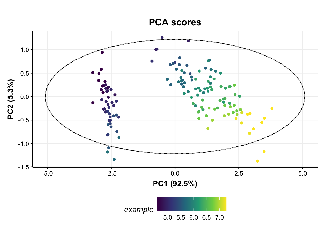


# scores plot
C1 = pca_scores_plot(factor_name='class') # colour by class
g1 = chart_plot(C1,M[2])

# scree plot
C2 = pca_scree_plot()
g2 = chart_plot(C2,M[2])

# arange in grid
grid.arrange(grobs=list(g1,g2),nrow=1)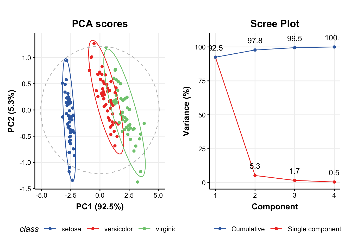

Typical workflow

Dataset

The MTBLS79 dataset represents a systematic evaluation of the reproducibility of a multi-batch direct-infusion mass spectrometry (DIMS)-based metabolomics study of cardiac tissue extracts. It comprises twenty biological samples (cow vs. sheep) that were analysed repeatedly, in 8 batches across 7 days, together with a concurrent set of quality control (QC) samples. Data are presented from each step of the data processing workflow and are available through MetaboLights (https://www.ebi.ac.uk/metabolights/MTBLS79).

# the pmp SE object
SE  <-  MTBLS79
# convert to DE
DE  <-  as.DatasetExperiment(SE)
DE$name  <-  "MTBLS79"
DE$description  <-  "Converted from SE provided by the pmp package"

# add a column indicating the order the samples were measured in
DE$sample_meta$run_order  <-  1:nrow(DE)

# add a column indicating if the sample is biological or a QC
Type <- as.character(DE$sample_meta$Class)
Type[Type != 'QC']  <-  "Sample"
DE$sample_meta$Type  <-  factor(Type)

# convert to factors
DE$sample_meta$Batch = factor(DE$sample_meta$Batch)
DE$sample_meta$Class = factor(DE$sample_meta$Class)

# print summary
DE
## A "DatasetExperiment" object
## ----------------------------
## name:          MTBLS79
## description:   Converted from SE provided by the pmp package
## data:          172 rows x 2488 columns
## sample_meta:   172 rows x 6 columns
## variable_meta: 2488 rows x 0 columns

Signal drift and batch correction

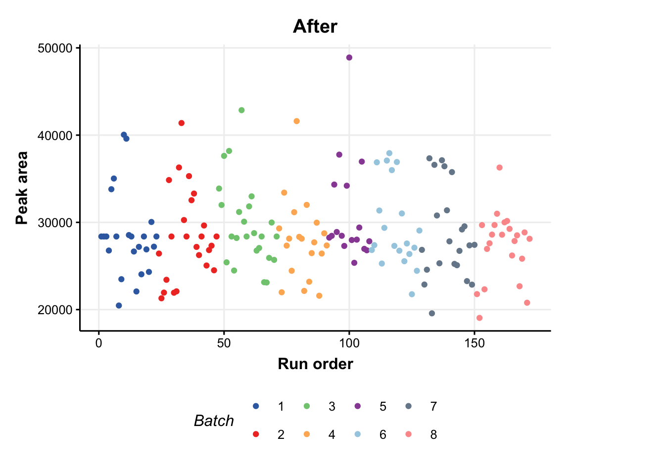
A batch correction algorithm is applied to reduce intra- and inter- batch variations in the dataset. Quality Control-Robust Spline Correction (QC-RSC) is provided in the pmp package, and it has been wrapped into a structToolbox object called sb_corr.

 # batch correction
M <- sb_corr(
    order_col = "run_order",
    batch_col = "Batch",
    qc_col = "Type",
    qc_label = "QC"
)

M = model_apply(M, DE)
## The number of NA and <= 0 values in peaksData before QC-RSC: 18222

### plot of a feature vs run order, before and after the correction
C = feature_profile(
      run_order='run_order',
      qc_label='QC',
      qc_column='Type',
      colour_by='Batch',
      feature_to_plot='200.03196'
  )

# plot and modify using ggplot2 
chart_plot(C,DE) + ylab('Peak area') + ggtitle('Before')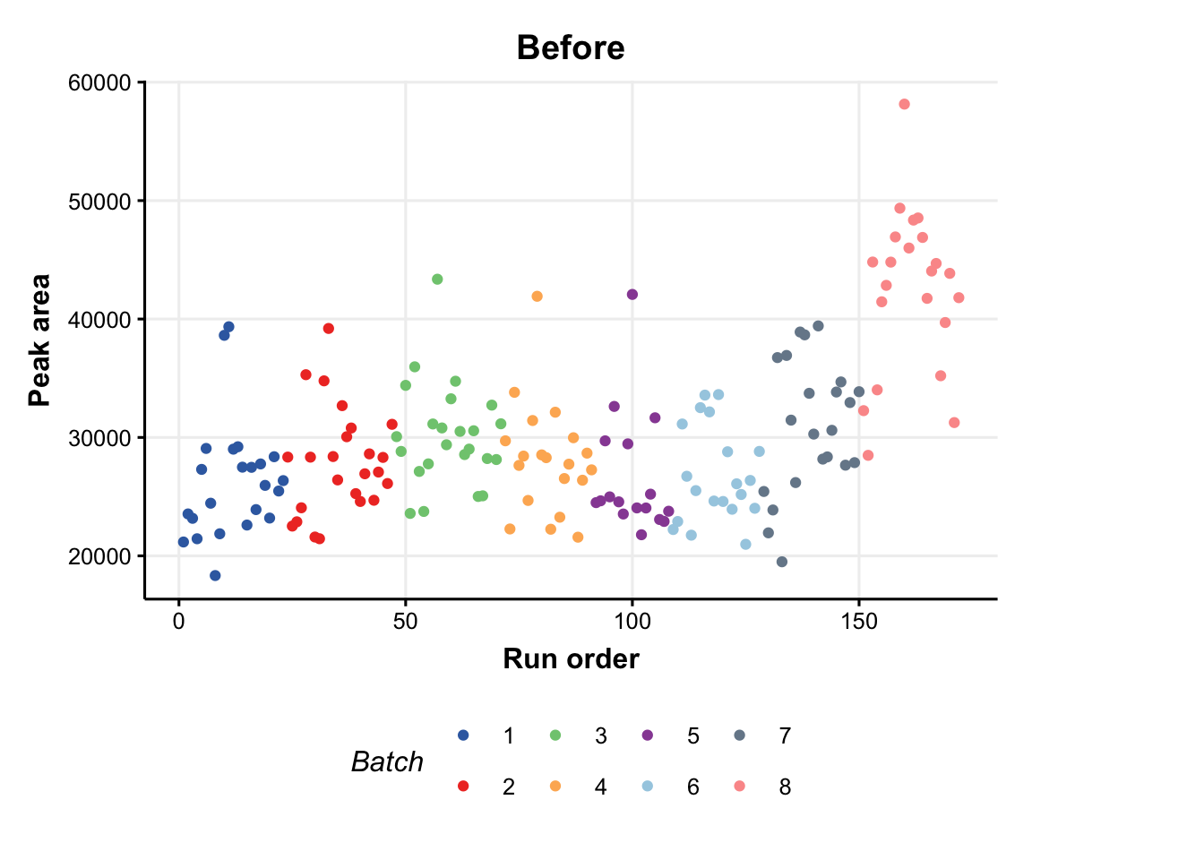


chart_plot(C,predicted(M))+ylab('Peak area')+ggtitle('After')


M2 = filter_na_count(
      threshold=3,
      factor_name='Batch'
    )
M2 = model_apply(M2,predicted(M))

# calculate number of features removed
nc = ncol(DE) - ncol(predicted(M2))

cat(paste0('Number of features removed: ', nc))
## Number of features removed: 425

Feature filtering

Reference

Data analysis of metabolomics and other omics datasets using the structToolbox