A sample example to add p-value and significant level to barpot.
Single group
stat.test <- ToothGrowth %>%
    t_test(data = ., len ~ dose, ref.group = "0.5") %>%
    mutate(p.adj.signif = replace_na(p.adj.signif, ""), across("p.adj.signif", str_replace, "ns", "")) %>%
    select(group1, group2, p.adj, p.adj.signif) %>%
    left_join(., df, by = c("group2" = "dose")) %>%
    mutate(y.position = value_mean + sd + 0.3)
## Warning: There was 1 warning in `mutate()`.
## ℹ In argument: `across("p.adj.signif", str_replace, "ns", "")`.
## Caused by warning:
## ! The `...` argument of `across()` is deprecated as of dplyr 1.1.0.
## Supply arguments directly to `.fns` through an anonymous function instead.
##
##   # Previously
##   across(a:b, mean, na.rm = TRUE)
##
##   # Now
##   across(a:b, \(x) mean(x, na.rm = TRUE))
theme_niwot <- function() {
theme_minimal() +
theme(
axis.title.x = element_blank(),
axis.line = element_line(color = "#3D4852"),
axis.ticks = element_line(color = "#3D4852"),
panel.grid.major.y = element_line(color = "#DAE1E7"),
panel.grid.major.x = element_blank(),
panel.background = element_rect(fill = "white"),
plot.background = element_rect(fill = "white"),
plot.margin = unit(rep(0.2, 4), "cm"),
axis.text = element_text(size = 12, color = "#22292F"),
axis.title = element_text(size = 12, hjust = 1),
axis.title.y = element_text(margin = margin(r = 12)),
axis.text.y = element_text(margin = margin(r = 5)),
axis.text.x = element_text(margin = margin(t = 5)),
legend.position = "non"
)
}df %>% ggplot(., aes(dose, value_mean)) +
geom_errorbar(aes(ymax = value_mean + sd, ymin = value_mean - sd), width = 0.1, color = "grey30") +
geom_col(width = 0.4, aes(fill = dose)) +
add_pvalue(stat.test,
label = "p.adj.signif", label.size = 6,
coord.flip = TRUE, remove.bracket = TRUE
) +
scale_y_continuous(expand = c(0, 0), limits = c(0, 33)) +
theme_niwot() +
scale_fill_brewer(palette = "Blues")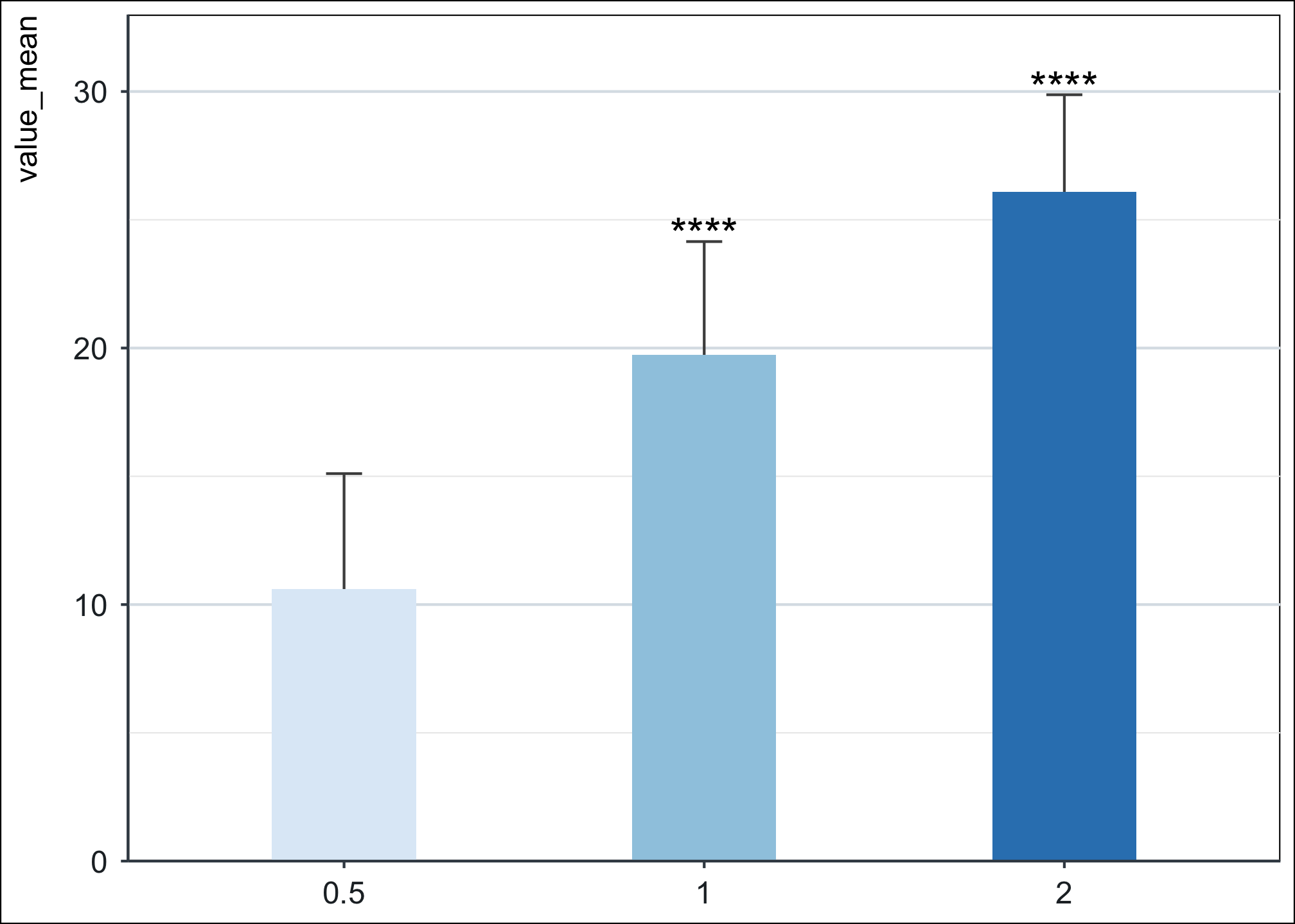
 df %>% ggplot(., aes(dose, value_mean)) +
     geom_errorbar(aes(ymax = value_mean + sd, ymin = value_mean - sd), width = 0.1, color = "grey30") +
     geom_col(width = 0.4, aes(fill = dose)) +
     stat_pvalue_manual(stat.test %>% slice(1),
         label = "p.adj.signif",
         label.size = 6, tip.length = c(0.35, 0.003), linetype = 2
     ) +
     add_pvalue(stat.test %>% slice(2), label = "p.adj.signif", label.size = 6, tip.length = c(0.1, 0.003)) +
     scale_y_continuous(expand = c(0, 0), limits = c(0, 33)) +
     theme_niwot() +
     scale_fill_brewer(palette = "Blues")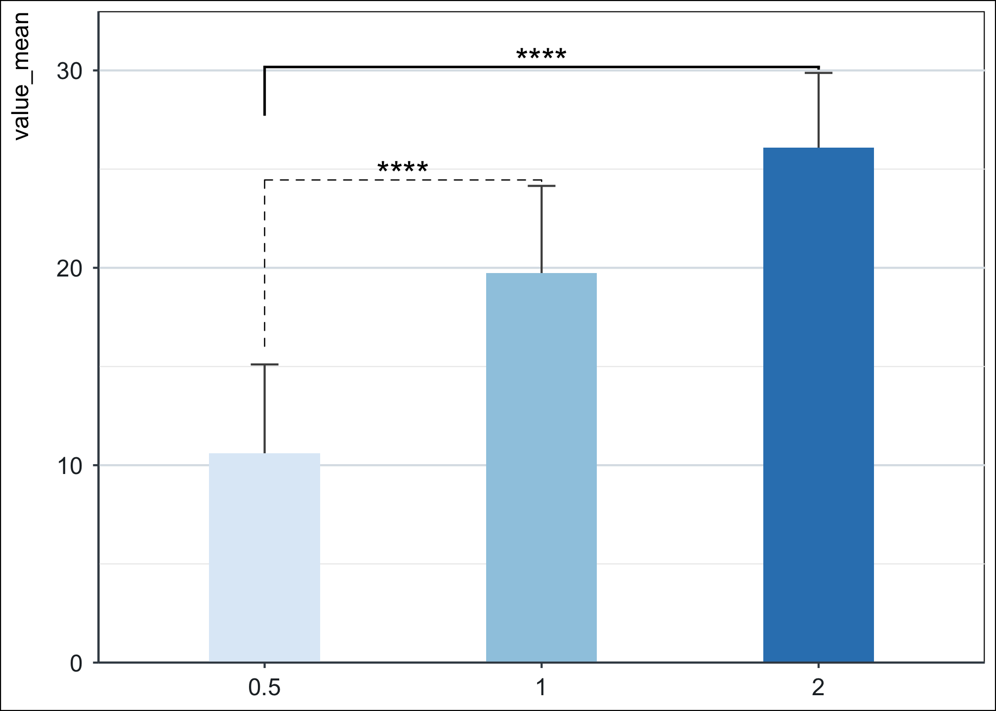
# ggsave(
# here("blog", "2023", "03", "06", "plot.png")
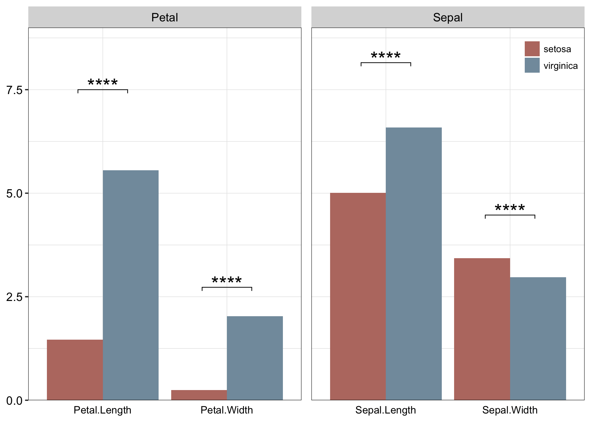
# )Multiple group
stat.test <- iris %>%
    pivot_longer(-Species) %>%
    filter(Species != "versicolor") %>%
    mutate(group = str_sub(name, start = 1, end = 5)) %>%
    group_by(group, name) %>%
    t_test(value ~ Species) %>%
    adjust_pvalue() %>%
    add_significance("p.adj") %>%
    add_xy_position(x = "name", scales = "free", fun = "max") %>%
    select(-3, -6, -7, -8, -9, -10) %>%
    mutate(
        across("xmin", str_replace, "2.8", "0.8"),
        across("xmin", str_replace, "3.8", "1.8"),
        across("xmax", str_replace, "3.2", "1.2"),
        across("xmax", str_replace, "4.2", "2.2")
    ) %>%
    mutate(xmin = as.numeric(xmin), xmax = as.numeric(xmax))

stat.test
## # A tibble: 4 × 11
##   name   group group1 group2    p.adj p.adj.signif y.position groups     x  xmin
##   <chr>  <chr> <chr>  <chr>     <dbl> <chr>             <dbl> <name> <dbl> <dbl>
## 1 Petal… Petal setosa virgi… 3.71e-49 ****               7.5  <chr>      1   0.8
## 2 Petal… Petal setosa virgi… 7.32e-48 ****               2.73 <chr>      2   1.8
## 3 Sepal… Sepal setosa virgi… 7.94e-25 ****               8.15 <chr>      3   0.8
## 4 Sepal… Sepal setosa virgi… 4.57e- 9 ****               4.47 <chr>      4   1.8
## # ℹ 1 more variable: xmax <dbl>
iris %>%
pivot_longer(-Species) %>%
filter(Species != "versicolor") %>%
mutate(group = str_sub(name, start = 1, end = 5)) %>%
ggplot(., aes(x = name, y = value)) +
stat_summary(geom = "bar", position = "dodge", aes(fill = Species)) +
stat_summary(
geom = "errorbar", fun.data = "mean_sdl",
fun.args = list(mult = 1),
aes(fill = Species),
position = position_dodge(0.9), width = 0.2, color = "black"
) +
stat_pvalue_manual(stat.test,
label = "p.adj.signif", label.size = 6, hide.ns = T,
tip.length = 0.01
) +
facet_wrap(. ~ group, scale = "free_x", nrow = 1) +
labs(x = NULL, y = NULL) +
scale_fill_manual(values = c("#BA7A70", "#829BAB")) +
scale_y_continuous(limits = c(0, 9), expand = c(0, 0)) +
theme(
axis.title.x = element_blank(),
axis.title.y = element_text(color = "black", size = 12, margin = margin(r = 3)),
axis.ticks.x = element_blank(),
axis.text.y = element_text(color = "black", size = 10, margin = margin(r = 2)),
axis.text.x = element_text(color = "black"),
panel.background = element_rect(fill = NA, color = NA),
panel.grid.minor = element_line(size = 0.2, color = "#e5e5e5"),
panel.grid.major = element_line(size = 0.2, color = "#e5e5e5"),
panel.border = element_rect(fill = NA, color = "black", size = 0.3, linetype = "solid"),
legend.key = element_blank(),
legend.title = element_blank(),
legend.text = element_text(color = "black", size = 8),
legend.spacing.x = unit(0.1, "cm"),
legend.key.width = unit(0.5, "cm"),
legend.key.height = unit(0.5, "cm"),
legend.position = c(1, 1), legend.justification = c(1, 1),
legend.background = element_blank(),
legend.box.margin = margin(0, 0, 0, 0),
strip.text = element_text(color = "black", size = 10),
panel.spacing.x = unit(0.3, "cm")
)
## Warning in stat_summary(geom = "errorbar", fun.data = "mean_sdl", fun.args =
## list(mult = 1), : Ignoring unknown aesthetics: fill
## Warning: The `size` argument of `element_rect()` is deprecated as of ggplot2 3.4.0.
## ℹ Please use the `linewidth` argument instead.
## Warning: The `size` argument of `element_line()` is deprecated as of ggplot2 3.4.0.
## ℹ Please use the `linewidth` argument instead.
## No summary function supplied, defaulting to `mean_se()`
## No summary function supplied, defaulting to `mean_se()`
## Warning: Computation failed in `stat_summary()`
## Caused by error in `fun.data()`:
## ! The package "Hmisc" is required.
## Warning: Computation failed in `stat_summary()`
## Caused by error in `fun.data()`:
## ! The package "Hmisc" is required.